Bayesian Logistic Regression Analysis
Description
This script uses inferential statistics to understand UFC fight odds data.
Libraries
library(tidyverse)
library(psych)
library(corrplot)
library(knitr)
library(Amelia)
library(rstanarm)
Examine Data
Load data.
load("./Datasets/df_master.RData")
Set the minimum number of fights required for a fighter to be included in the analysis.
fight_min = 1
Summarize data.
summary(df_master)

##      NAME               Date              Event               City
##  Length:6088        Length:6088        Length:6088        Length:6088
##  Class :character   Class :character   Class :character   Class :character
##  Mode  :character   Mode  :character   Mode  :character   Mode  :character
##
##
##
##
##     State             Country          FightWeightClass       Round
##  Length:6088        Length:6088        Length:6088        Min.   :1.000
##  Class :character   Class :character   Class :character   1st Qu.:1.000
##  Mode  :character   Mode  :character   Mode  :character   Median :3.000
##                                                           Mean   :2.431
##                                                           3rd Qu.:3.000
##                                                           Max.   :5.000
##
##     Method          Winner_Odds         Loser_Odds            Sex
##  Length:6088        Length:6088        Length:6088        Length:6088
##  Class :character   Class :character   Class :character   Class :character
##  Mode  :character   Mode  :character   Mode  :character   Mode  :character
##
##
##
##
##     fight_id         Result          FighterWeight   FighterWeightClass
##  Min.   :   1.0   Length:6088        Min.   :115.0   Length:6088
##  1st Qu.: 761.8   Class :character   1st Qu.:135.0   Class :character
##  Median :1522.5   Mode  :character   Median :155.0   Mode  :character
##  Mean   :1522.5                      Mean   :163.9
##  3rd Qu.:2283.2                      3rd Qu.:185.0
##  Max.   :3044.0                      Max.   :265.0
##
##      REACH            SLPM             SAPM             STRA
##  Min.   :58.00   Min.   : 0.000   Min.   : 0.100   Min.   :0.0000
##  1st Qu.:69.00   1st Qu.: 2.680   1st Qu.: 2.630   1st Qu.:0.3900
##  Median :72.00   Median : 3.440   Median : 3.240   Median :0.4400
##  Mean   :71.77   Mean   : 3.529   Mean   : 3.434   Mean   :0.4422
##  3rd Qu.:75.00   3rd Qu.: 4.220   3rd Qu.: 4.020   3rd Qu.:0.4900
##  Max.   :84.00   Max.   :19.910   Max.   :21.180   Max.   :0.8800
##  NA's   :215
##       STRD              TD             TDA              TDD
##  Min.   :0.0900   Min.   :0.000   Min.   :0.0000   Min.   :0.0000
##  1st Qu.:0.5100   1st Qu.:0.560   1st Qu.:0.2600   1st Qu.:0.5100
##  Median :0.5600   Median :1.210   Median :0.3700   Median :0.6400
##  Mean   :0.5516   Mean   :1.520   Mean   :0.3752   Mean   :0.6158
##  3rd Qu.:0.6000   3rd Qu.:2.183   3rd Qu.:0.5000   3rd Qu.:0.7600
##  Max.   :0.9200   Max.   :8.930   Max.   :1.0000   Max.   :1.0000
##
##       SUBA
##  Min.   : 0.0000
##  1st Qu.: 0.1000
##  Median : 0.4000
##  Mean   : 0.5506
##  3rd Qu.: 0.8000
##  Max.   :12.1000
##
Redefine variables.
df_master$NAME = as.factor(df_master$NAME)
df_master$Date = as.Date(df_master$Date)
df_master$Event = as.factor(df_master$Event)
df_master$City= as.factor(df_master$City)
df_master$State = as.factor(df_master$State)
df_master$Country = as.factor(df_master$Country)
df_master$FightWeightClass = as.factor(df_master$FightWeightClass)
# will keep round as integer since represents time in match...
# df_master$Round = as.factor(df_master$Round)
df_master$Method = as.factor(df_master$Method)
df_master$Winner_Odds = as.numeric(df_master$Winner_Odds)
df_master$Loser_Odds = as.numeric(df_master$Loser_Odds)
df_master$fight_id = as.factor(df_master$fight_id)
df_master$Sex = as.factor(df_master$Sex)
df_master$Result = as.factor(df_master$Result)
df_master$FighterWeightClass = as.factor(df_master$FighterWeightClass)
Summarize again. There are infinite odds and overturned / DQ fight outcomes. These will have to be removed.
summary(df_master)

##                  NAME           Date
##  Donald Cerrone    :  24   Min.   :2013-04-27
##  Ovince Saint Preux:  21   1st Qu.:2015-09-05
##  Jim Miller        :  20   Median :2017-06-17
##  Derrick Lewis     :  19   Mean   :2017-07-11
##  Neil Magny        :  19   3rd Qu.:2019-05-18
##  Andrei Arlovski   :  18   Max.   :2021-04-17
##  (Other)           :5967
##                                   Event                  City
##  UFC 259: Blachowicz vs. Adesanya    :  30   Las Vegas     :1346
##  UFC Fight Night: Chiesa vs. Magny   :  28   Abu Dhabi     : 258
##  UFC Fight Night: Poirier vs. Gaethje:  28   Boston        : 124
##  UFC Fight Night: Whittaker vs. Till :  28   Rio de Janeiro: 124
##  UFC 190: Rousey vs Correia          :  26   Chicago       : 118
##  UFC 193: Rousey vs Holm             :  26   Newark        : 114
##  (Other)                             :5922   (Other)       :4004
##         State                      Country          FightWeightClass
##  Nevada    :1346   USA                 :3564   Lightweight  : 998
##  Abu Dhabi : 258   Brazil              : 534   Welterweight : 992
##  Texas     : 256   Canada              : 378   Bantamweight : 872
##  New York  : 252   United Arab Emirates: 258   Featherweight: 736
##  California: 250   Australia           : 236   Middleweight : 666
##  Florida   : 176   United Kingdom      : 184   Flyweight    : 508
##  (Other)   :3550   (Other)             : 934   (Other)      :1316
##      Round              Method      Winner_Odds     Loser_Odds       Sex
##  Min.   :1.000   DQ        :  16   Min.   :1.06   Min.   :1.07   Female: 780
##  1st Qu.:1.000   KO/TKO    :1940   1st Qu.:1.42   1st Qu.:1.77   Male  :5308
##  Median :3.000   M-DEC     :  36   Median :1.71   Median :2.38
##  Mean   :2.431   Overturned:  20   Mean   : Inf   Mean   : Inf
##  3rd Qu.:3.000   S-DEC     : 642   3rd Qu.:2.33   3rd Qu.:3.35
##  Max.   :5.000   SUB       :1078   Max.   : Inf   Max.   : Inf
##                  U-DEC     :2356
##     fight_id       Result     FighterWeight       FighterWeightClass
##  1      :   2   Loser :3044   Min.   :115.0   Welterweight :1018
##  2      :   2   Winner:3044   1st Qu.:135.0   Lightweight  : 992
##  3      :   2                 Median :155.0   Bantamweight : 821
##  4      :   2                 Mean   :163.9   Featherweight: 739
##  5      :   2                 3rd Qu.:185.0   Middleweight : 667
##  6      :   2                 Max.   :265.0   Flyweight    : 570
##  (Other):6076                                 (Other)      :1281
##      REACH            SLPM             SAPM             STRA
##  Min.   :58.00   Min.   : 0.000   Min.   : 0.100   Min.   :0.0000
##  1st Qu.:69.00   1st Qu.: 2.680   1st Qu.: 2.630   1st Qu.:0.3900
##  Median :72.00   Median : 3.440   Median : 3.240   Median :0.4400
##  Mean   :71.77   Mean   : 3.529   Mean   : 3.434   Mean   :0.4422
##  3rd Qu.:75.00   3rd Qu.: 4.220   3rd Qu.: 4.020   3rd Qu.:0.4900
##  Max.   :84.00   Max.   :19.910   Max.   :21.180   Max.   :0.8800
##  NA's   :215
##       STRD              TD             TDA              TDD
##  Min.   :0.0900   Min.   :0.000   Min.   :0.0000   Min.   :0.0000
##  1st Qu.:0.5100   1st Qu.:0.560   1st Qu.:0.2600   1st Qu.:0.5100
##  Median :0.5600   Median :1.210   Median :0.3700   Median :0.6400
##  Mean   :0.5516   Mean   :1.520   Mean   :0.3752   Mean   :0.6158
##  3rd Qu.:0.6000   3rd Qu.:2.183   3rd Qu.:0.5000   3rd Qu.:0.7600
##  Max.   :0.9200   Max.   :8.930   Max.   :1.0000   Max.   :1.0000
##
##       SUBA
##  Min.   : 0.0000
##  1st Qu.: 0.1000
##  Median : 0.4000
##  Mean   : 0.5506
##  3rd Qu.: 0.8000
##  Max.   :12.1000
##
How many events are there in the dataset?
length(unique(df_master$Event))

## [1] 265
How many fights?
length(unique(df_master$fight_id))

## [1] 3044
Over what time frame did these occur?
range(sort(unique(df_master$Date)))

## [1] "2013-04-27" "2021-04-17"
Preprocess Data
Make copy of data frame.
df_stats = df_master
Calculate number of fights in dataset for each fighter in dataset.
df_stats %>%
  dplyr::group_by(NAME) %>%
  dplyr::summarise(
    Num_Fights = length(Round)
  ) -> df_fight_count
Append fight count to dataframe.
df_stats = merge(df_stats, df_fight_count)
Which fights will we lose due to equal odds?
df_stats %>%
  dplyr::filter(Winner_Odds == Loser_Odds) -> df_equal_odds

kable(df_equal_odds)
| NAME | Date | Event | City | State | Country | FightWeightClass | Round | Method | Winner_Odds | Loser_Odds | Sex | fight_id | Result | FighterWeight | FighterWeightClass | REACH | SLPM | SAPM | STRA | STRD | TD | TDA | TDD | SUBA | Num_Fights |
|---|---|---|---|---|---|---|---|---|---|---|---|---|---|---|---|---|---|---|---|---|---|---|---|---|---|
| Abdul Razak Alhassan | 2021-04-17 | UFC Fight Night: Whittaker vs. Gastelum | Las Vegas | Nevada | USA | Middleweight | 3 | U-DEC | Inf | Inf | Male | 1220 | Loser | 170 | Welterweight | 73 | 3.71 | 4.24 | 0.47 | 0.53 | 0.53 | 0.28 | 0.55 | 0.0 | 7 |
| Aisling Daly | 2015-10-24 | UFC Fight Night: Holohan vs Smolka | Dublin | Leinster | Ireland | Strawweight | 3 | U-DEC | 2.00 | 2.00 | Female | 18 | Winner | 115 | Strawweight | 64 | 2.92 | 1.40 | 0.52 | 0.55 | 2.15 | 0.41 | 0.33 | 0.9 | 3 |
| Aleksei Oleinik | 2017-11-04 | UFC 217: Bisping vs. St-Pierre | New York City | New York | USA | Heavyweight | 2 | KO/TKO | Inf | Inf | Male | 617 | Loser | 240 | Heavyweight | 80 | 3.47 | 3.85 | 0.50 | 0.44 | 2.38 | 0.46 | 0.33 | 2.4 | 14 |
| Aleksei Oleinik | 2017-07-08 | UFC 213: Romero vs. Whittaker | Las Vegas | Nevada | USA | Heavyweight | 2 | SUB | Inf | Inf | Male | 62 | Winner | 240 | Heavyweight | 80 | 3.47 | 3.85 | 0.50 | 0.44 | 2.38 | 0.46 | 0.33 | 2.4 | 14 |
| Ali AlQaisi | 2020-10-10 | UFC Fight Night: Moraes vs. Sandhagen | Abu Dhabi | Abu Dhabi | United Arab Emirates | Bantamweight | 3 | U-DEC | Inf | Inf | Male | 2694 | Loser | 135 | Bantamweight | 68 | 2.43 | 1.97 | 0.42 | 0.56 | 3.50 | 0.29 | 0.60 | 1.0 | 2 |
| Alvaro Herrera Mendoza | 2018-07-28 | UFC Fight Night: Alvarez vs. Poirier 2 | Calgary | Alberta | Canada | Lightweight | 1 | KO/TKO | 2.00 | 2.00 | Male | 801 | Loser | 155 | Lightweight | 74 | 1.89 | 3.40 | 0.38 | 0.55 | 0.00 | 0.00 | 0.33 | 1.1 | 2 |
| Anthony Johnson | 2015-05-23 | UFC 187: Johnson vs Cormier | Las Vegas | Nevada | USA | Light Heavyweight | 3 | SUB | 1.96 | 1.96 | Male | 655 | Loser | 205 | Light Heavyweight | 78 | 3.25 | 1.83 | 0.47 | 0.60 | 2.43 | 0.57 | 0.77 | 0.6 | 8 |
| Antonio Carlos Junior | 2017-10-28 | UFC Fight Night: Brunson vs. Machida | Sao Paulo | Sao Paulo | Brazil | Middleweight | 1 | SUB | Inf | Inf | Male | 251 | Winner | 185 | Middleweight | 79 | 1.95 | 2.14 | 0.42 | 0.52 | 3.42 | 0.39 | 0.53 | 0.8 | 9 |
| Ariane Lipski | 2019-11-16 | UFC Fight Night: Blachowicz vs. Jacare | Sao Paulo | Sao Paulo | Brazil | Flyweight | 3 | U-DEC | Inf | Inf | Female | 254 | Winner | 125 | Flyweight | 67 | 3.03 | 4.45 | 0.32 | 0.48 | 0.27 | 0.25 | 0.45 | 0.5 | 4 |
| Bevon Lewis | 2018-12-29 | UFC 232: Jones vs. Gustafsson 2 | Los Angeles | California | USA | Middleweight | 3 | KO/TKO | Inf | Inf | Male | 2881 | Loser | 185 | Middleweight | 79 | 3.73 | 2.67 | 0.43 | 0.54 | 0.00 | 0.00 | 0.66 | 0.0 | 3 |
| Brian Camozzi | 2018-02-18 | UFC Fight Night: Cerrone vs. Medeiros | Austin | Texas | USA | Welterweight | 1 | SUB | Inf | Inf | Male | 1041 | Loser | 170 | Welterweight | 78 | 3.15 | 6.39 | 0.26 | 0.54 | 0.00 | 0.00 | 0.00 | 0.7 | 3 |
| Carlos Condit | 2016-01-02 | UFC 195: Lawler vs Condit | Las Vegas | Nevada | USA | Welterweight | 5 | S-DEC | 1.95 | 1.95 | Male | 2336 | Loser | 170 | Welterweight | 75 | 3.63 | 2.49 | 0.39 | 0.56 | 0.62 | 0.54 | 0.39 | 1.0 | 8 |
| Carlton Minus | 2020-08-22 | UFC Fight Night: Munhoz vs. Edgar | Las Vegas | Nevada | USA | Welterweight | 3 | U-DEC | Inf | Inf | Male | 2887 | Loser | 170 | Welterweight | 75 | 3.50 | 4.97 | 0.40 | 0.50 | 0.00 | 0.00 | 0.58 | 0.0 | 2 |
| Cezar Ferreira | 2018-05-12 | UFC 224: Nunes vs. Pennington | Rio de Janeiro | Rio de Janeiro | Brazil | Middleweight | 1 | SUB | 1.95 | 1.95 | Male | 453 | Winner | 185 | Middleweight | 78 | 1.90 | 2.44 | 0.42 | 0.53 | 2.69 | 0.53 | 0.84 | 0.5 | 13 |
| Curtis Blaydes | 2017-11-04 | UFC 217: Bisping vs. St-Pierre | New York City | New York | USA | Heavyweight | 2 | KO/TKO | Inf | Inf | Male | 617 | Winner | 265 | Heavyweight | 80 | 3.59 | 1.70 | 0.53 | 0.57 | 6.64 | 0.54 | 0.33 | 0.0 | 12 |
| Da-Un Jung | 2021-04-10 | UFC Fight Night: Vettori vs. Holland | Las Vegas | Nevada | USA | Light Heavyweight | 3 | U-DEC | Inf | Inf | Male | 3039 | Winner | 205 | Light Heavyweight | 78 | 3.95 | 3.90 | 0.45 | 0.54 | 2.79 | 0.61 | 0.88 | 0.3 | 3 |
| Daniel Cormier | 2015-05-23 | UFC 187: Johnson vs Cormier | Las Vegas | Nevada | USA | Light Heavyweight | 3 | SUB | 1.96 | 1.96 | Male | 655 | Winner | 235 | Heavyweight | 72 | 4.25 | 2.92 | 0.52 | 0.54 | 1.83 | 0.44 | 0.80 | 0.4 | 10 |
| Darrick Minner | 2020-09-19 | UFC Fight Night: Covington vs. Woodley | Las Vegas | Nevada | USA | Featherweight | 1 | SUB | Inf | Inf | Male | 715 | Winner | 145 | Featherweight | 69 | 3.24 | 1.40 | 0.70 | 0.43 | 3.00 | 0.62 | 0.60 | 3.6 | 3 |
| Deiveson Figueiredo | 2018-02-03 | UFC Fight Night: Machida vs. Anders | Belem | Para | Brazil | Flyweight | 2 | KO/TKO | 2.20 | 2.20 | Male | 734 | Winner | 125 | Flyweight | 68 | 3.38 | 3.35 | 0.56 | 0.50 | 1.57 | 0.50 | 0.61 | 2.4 | 8 |
| Devin Powell | 2018-07-28 | UFC Fight Night: Alvarez vs. Poirier 2 | Calgary | Alberta | Canada | Lightweight | 1 | KO/TKO | 2.00 | 2.00 | Male | 801 | Winner | 155 | Lightweight | 73 | 2.88 | 3.67 | 0.41 | 0.51 | 0.00 | 0.00 | 0.00 | 0.6 | 4 |
| Devonte Smith | 2019-02-09 | UFC 234: Adesanya vs. Silva | Melbourne | Victoria | Australia | Lightweight | 1 | KO/TKO | Inf | Inf | Male | 803 | Winner | 155 | Lightweight | 76 | 5.64 | 2.65 | 0.55 | 0.59 | 0.74 | 1.00 | 1.00 | 0.7 | 4 |
| Dong Hyun Ma | 2019-02-09 | UFC 234: Adesanya vs. Silva | Melbourne | Victoria | Australia | Lightweight | 1 | KO/TKO | Inf | Inf | Male | 803 | Loser | 155 | Lightweight | 70 | 2.84 | 4.10 | 0.41 | 0.54 | 1.27 | 0.53 | 0.33 | 0.0 | 8 |
| Dong Hyun Ma | 2017-09-22 | UFC Fight Night: Saint Preux vs. Okami | Saitama | Saitama | Japan | Lightweight | 1 | KO/TKO | Inf | Inf | Male | 849 | Winner | 155 | Lightweight | 70 | 2.84 | 4.10 | 0.41 | 0.54 | 1.27 | 0.53 | 0.33 | 0.0 | 8 |
| Ericka Almeida | 2015-10-24 | UFC Fight Night: Holohan vs Smolka | Dublin | Leinster | Ireland | Strawweight | 3 | U-DEC | 2.00 | 2.00 | Female | 18 | Loser | 115 | Strawweight | NA | 1.07 | 3.33 | 0.39 | 0.43 | 0.50 | 0.33 | 0.37 | 0.0 | 2 |
| Felicia Spencer | 2020-02-29 | UFC Fight Night: Benavidez vs. Figueiredo | Norfolk | Virginia | USA | Featherweight | 1 | KO/TKO | Inf | Inf | Female | 974 | Winner | 145 | Featherweight | 68 | 3.02 | 5.57 | 0.45 | 0.43 | 0.64 | 0.10 | 0.14 | 0.3 | 4 |
| Felipe Colares | 2019-02-02 | UFC Fight Night: Assuncao vs. Moraes 2 | Fortaleza | Ceara | Brazil | Featherweight | 3 | U-DEC | Inf | Inf | Male | 2915 | Loser | 135 | Bantamweight | 69 | 1.13 | 3.00 | 0.42 | 0.32 | 2.00 | 0.25 | 0.34 | 1.0 | 3 |
| Frankie Perez | 2015-01-18 | UFC Fight Night: McGregor vs Siver | Boston | Massachusetts | USA | Lightweight | 3 | KO/TKO | Inf | Inf | Male | 1432 | Loser | 155 | Lightweight | 73 | 1.64 | 2.17 | 0.41 | 0.54 | 1.75 | 0.41 | 0.50 | 0.3 | 4 |
| Frankie Saenz | 2018-05-19 | UFC Fight Night: Maia vs. Usman | Santiago | Chile | Chile | Bantamweight | 3 | U-DEC | Inf | Inf | Male | 1021 | Winner | 135 | Bantamweight | 66 | 3.94 | 3.50 | 0.47 | 0.52 | 1.74 | 0.31 | 0.61 | 0.1 | 9 |
| Geoff Neal | 2018-02-18 | UFC Fight Night: Cerrone vs. Medeiros | Austin | Texas | USA | Welterweight | 1 | SUB | Inf | Inf | Male | 1041 | Winner | 170 | Welterweight | 75 | 4.94 | 4.93 | 0.49 | 0.61 | 0.50 | 0.50 | 0.92 | 0.2 | 5 |
| Geraldo de Freitas | 2019-02-02 | UFC Fight Night: Assuncao vs. Moraes 2 | Fortaleza | Ceara | Brazil | Featherweight | 3 | U-DEC | Inf | Inf | Male | 2915 | Winner | 135 | Bantamweight | 72 | 3.67 | 2.62 | 0.52 | 0.50 | 3.00 | 0.45 | 0.59 | 0.0 | 3 |
| Gina Mazany | 2017-11-25 | UFC Fight Night: Bisping vs. Gastelum | Shanghai | Hebei | China | Bantamweight | 3 | U-DEC | 2.25 | 2.25 | Female | 1087 | Winner | 125 | Flyweight | 68 | 3.45 | 3.07 | 0.47 | 0.51 | 4.41 | 0.63 | 0.33 | 0.3 | 6 |
| Glover Teixeira | 2015-08-08 | UFC Fight Night: Teixeira vs Saint Preux | Nashville | Tennessee | USA | Light Heavyweight | 3 | SUB | 1.95 | 1.95 | Male | 1093 | Winner | 205 | Light Heavyweight | 76 | 3.75 | 3.84 | 0.47 | 0.54 | 2.04 | 0.40 | 0.60 | 1.0 | 12 |
| Henry Briones | 2018-05-19 | UFC Fight Night: Maia vs. Usman | Santiago | Chile | Chile | Bantamweight | 3 | U-DEC | Inf | Inf | Male | 1021 | Loser | 135 | Bantamweight | 69 | 3.47 | 4.68 | 0.42 | 0.53 | 0.00 | 0.00 | 0.52 | 0.6 | 4 |
| Ildemar Alcantara | 2015-07-15 | UFC Fight Night: Mir vs Duffee | San Diego | California | USA | Middleweight | 3 | U-DEC | 1.95 | 1.95 | Male | 1624 | Loser | 185 | Middleweight | 78 | 1.93 | 2.63 | 0.38 | 0.50 | 2.00 | 0.68 | 0.81 | 0.9 | 3 |
| Isabela de Padua | 2019-11-16 | UFC Fight Night: Blachowicz vs. Jacare | Sao Paulo | Sao Paulo | Brazil | Flyweight | 3 | U-DEC | Inf | Inf | Female | 254 | Loser | 125 | Flyweight | 64 | 1.00 | 2.07 | 0.35 | 0.50 | 2.00 | 0.66 | 0.00 | 1.0 | 1 |
| Iuri Alcantara | 2018-02-03 | UFC Fight Night: Machida vs. Anders | Belem | Para | Brazil | Bantamweight | 1 | KO/TKO | 2.00 | 2.00 | Male | 2949 | Winner | 135 | Bantamweight | 71 | 2.72 | 2.79 | 0.45 | 0.49 | 1.44 | 0.62 | 0.60 | 0.8 | 12 |
| Jack Marshman | 2017-10-28 | UFC Fight Night: Brunson vs. Machida | Sao Paulo | Sao Paulo | Brazil | Middleweight | 1 | SUB | Inf | Inf | Male | 251 | Loser | 185 | Middleweight | 73 | 2.74 | 4.19 | 0.25 | 0.56 | 0.00 | 0.00 | 0.20 | 0.0 | 6 |
| Jacob Malkoun | 2021-04-17 | UFC Fight Night: Whittaker vs. Gastelum | Las Vegas | Nevada | USA | Middleweight | 3 | U-DEC | Inf | Inf | Male | 1220 | Winner | 185 | Middleweight | 73 | 1.76 | 1.83 | 0.47 | 0.51 | 7.84 | 0.33 | 0.00 | 2.0 | 2 |
| Jarjis Danho | 2021-04-10 | UFC Fight Night: Vettori vs. Holland | Las Vegas | Nevada | USA | Heavyweight | 1 | KO/TKO | Inf | Inf | Male | 1288 | Winner | 265 | Heavyweight | 74 | 3.38 | 5.25 | 0.50 | 0.49 | 0.51 | 0.16 | 1.00 | 0.0 | 2 |
| Joanne Calderwood | 2019-06-08 | UFC 238: Cejudo vs. Moraes | Chicago | Illinois | USA | Flyweight | 3 | U-DEC | 1.98 | 1.98 | Female | 1596 | Loser | 125 | Flyweight | 65 | 6.59 | 4.40 | 0.49 | 0.53 | 1.80 | 0.55 | 0.58 | 0.5 | 9 |
| Joe Soto | 2018-02-03 | UFC Fight Night: Machida vs. Anders | Belem | Para | Brazil | Bantamweight | 1 | KO/TKO | 2.00 | 2.00 | Male | 2949 | Loser | 135 | Bantamweight | 65 | 3.36 | 5.37 | 0.41 | 0.67 | 0.85 | 0.21 | 0.70 | 1.9 | 7 |
| Johnny Case | 2015-01-18 | UFC Fight Night: McGregor vs Siver | Boston | Massachusetts | USA | Lightweight | 3 | KO/TKO | Inf | Inf | Male | 1432 | Winner | 155 | Lightweight | 72 | 3.95 | 2.66 | 0.38 | 0.61 | 1.70 | 0.45 | 0.72 | 0.2 | 6 |
| Johny Hendricks | 2017-11-04 | UFC 217: Bisping vs. St-Pierre | New York City | New York | USA | Middleweight | 2 | KO/TKO | Inf | Inf | Male | 2198 | Loser | 185 | Middleweight | 69 | 3.49 | 3.99 | 0.45 | 0.53 | 3.83 | 0.46 | 0.63 | 0.3 | 9 |
| Jorge Masvidal | 2016-05-29 | UFC Fight Night: Almeida vs Garbrandt | Las Vegas | Nevada | USA | Welterweight | 3 | S-DEC | 2.00 | 2.00 | Male | 1750 | Loser | 170 | Welterweight | 74 | 4.20 | 3.00 | 0.47 | 0.65 | 1.57 | 0.59 | 0.77 | 0.4 | 15 |
| Joseph Morales | 2018-02-03 | UFC Fight Night: Machida vs. Anders | Belem | Para | Brazil | Flyweight | 2 | KO/TKO | 2.20 | 2.20 | Male | 734 | Loser | 125 | Flyweight | 69 | 1.58 | 1.72 | 0.37 | 0.60 | 0.53 | 0.50 | 0.23 | 2.6 | 2 |
| Karl Roberson | 2018-05-12 | UFC 224: Nunes vs. Pennington | Rio de Janeiro | Rio de Janeiro | Brazil | Middleweight | 1 | SUB | 1.95 | 1.95 | Male | 453 | Loser | 185 | Middleweight | 74 | 3.00 | 2.42 | 0.51 | 0.57 | 0.99 | 0.57 | 0.50 | 0.8 | 6 |
| Katlyn Chookagian | 2019-06-08 | UFC 238: Cejudo vs. Moraes | Chicago | Illinois | USA | Flyweight | 3 | U-DEC | 1.98 | 1.98 | Female | 1596 | Winner | 125 | Flyweight | 68 | 4.22 | 4.23 | 0.34 | 0.63 | 0.27 | 0.15 | 0.51 | 0.5 | 11 |
| KB Bhullar | 2020-10-10 | UFC Fight Night: Moraes vs. Sandhagen | Abu Dhabi | Abu Dhabi | United Arab Emirates | Middleweight | 1 | KO/TKO | Inf | Inf | Male | 2678 | Loser | 185 | Middleweight | 78 | 1.18 | 10.00 | 0.13 | 0.37 | 0.00 | 0.00 | 0.00 | 0.0 | 1 |
| Kevin Casey | 2015-07-15 | UFC Fight Night: Mir vs Duffee | San Diego | California | USA | Middleweight | 3 | U-DEC | 1.95 | 1.95 | Male | 1624 | Winner | 185 | Middleweight | 77 | 2.27 | 3.76 | 0.53 | 0.46 | 0.79 | 0.22 | 0.27 | 0.4 | 3 |
| Kyle Bochniak | 2019-10-18 | UFC Fight Night: Reyes vs. Weidman | Boston | Massachusetts | USA | Featherweight | 3 | U-DEC | 2.00 | 2.00 | Male | 2486 | Loser | 145 | Featherweight | 70 | 2.63 | 5.11 | 0.31 | 0.58 | 1.14 | 0.15 | 0.62 | 0.0 | 7 |
| Lorenz Larkin | 2016-05-29 | UFC Fight Night: Almeida vs Garbrandt | Las Vegas | Nevada | USA | Welterweight | 3 | S-DEC | 2.00 | 2.00 | Male | 1750 | Winner | 170 | Welterweight | 72 | 3.53 | 2.74 | 0.46 | 0.63 | 0.27 | 0.42 | 0.79 | 0.1 | 7 |
| Luis Pena | 2020-02-29 | UFC Fight Night: Benavidez vs. Figueiredo | Norfolk | Virginia | USA | Lightweight | 3 | U-DEC | Inf | Inf | Male | 1770 | Winner | 155 | Lightweight | 75 | 3.66 | 3.12 | 0.46 | 0.51 | 1.17 | 0.33 | 0.48 | 1.2 | 6 |
| Luke Sanders | 2018-08-25 | UFC Fight Night: Gaethje vs. Vick | Lincoln | Nebraska | USA | Bantamweight | 1 | SUB | 2.00 | 2.00 | Male | 2261 | Loser | 135 | Bantamweight | 67 | 6.21 | 4.11 | 0.51 | 0.53 | 0.31 | 0.20 | 0.66 | 0.3 | 6 |
| Magomed Mustafaev | 2019-04-20 | UFC Fight Night: Overeem vs. Oleinik | Saint Petersburg | Saint Petersburg | Russia | Lightweight | 1 | KO/TKO | 2.25 | 2.25 | Male | 1806 | Winner | 155 | Lightweight | 71 | 2.59 | 2.68 | 0.58 | 0.41 | 3.31 | 0.50 | 0.23 | 0.4 | 5 |
| Matthew Semelsberger | 2020-08-22 | UFC Fight Night: Munhoz vs. Edgar | Las Vegas | Nevada | USA | Welterweight | 3 | U-DEC | Inf | Inf | Male | 2887 | Winner | 170 | Welterweight | 75 | 7.93 | 5.31 | 0.50 | 0.56 | 1.97 | 1.00 | 1.00 | 1.0 | 1 |
| Misha Cirkunov | 2016-12-10 | UFC 206: Holloway vs. Pettis | Toronto | Ontario | Canada | Light Heavyweight | 1 | SUB | 1.88 | 1.88 | Male | 2047 | Winner | 205 | Light Heavyweight | 77 | 4.18 | 3.22 | 0.51 | 0.60 | 4.28 | 0.57 | 0.71 | 2.3 | 9 |
| Nikita Krylov | 2016-12-10 | UFC 206: Holloway vs. Pettis | Toronto | Ontario | Canada | Light Heavyweight | 1 | SUB | 1.88 | 1.88 | Male | 2047 | Loser | 205 | Light Heavyweight | 77 | 4.33 | 2.52 | 0.56 | 0.43 | 1.34 | 0.33 | 0.55 | 1.3 | 11 |
| Ovince Saint Preux | 2015-08-08 | UFC Fight Night: Teixeira vs Saint Preux | Nashville | Tennessee | USA | Light Heavyweight | 3 | SUB | 1.95 | 1.95 | Male | 1093 | Loser | 205 | Light Heavyweight | 80 | 2.68 | 3.03 | 0.46 | 0.45 | 1.19 | 0.40 | 0.66 | 0.6 | 21 |
| Paulo Costa | 2018-07-07 | UFC 226: Miocic vs. Cormier | Las Vegas | Nevada | USA | Middleweight | 2 | KO/TKO | Inf | Inf | Male | 2199 | Winner | 185 | Middleweight | 72 | 7.03 | 6.70 | 0.57 | 0.50 | 0.00 | 0.00 | 0.80 | 0.0 | 5 |
| Paulo Costa | 2017-11-04 | UFC 217: Bisping vs. St-Pierre | New York City | New York | USA | Middleweight | 2 | KO/TKO | Inf | Inf | Male | 2198 | Winner | 185 | Middleweight | 72 | 7.03 | 6.70 | 0.57 | 0.50 | 0.00 | 0.00 | 0.80 | 0.0 | 5 |
| Rafael Fiziev | 2019-04-20 | UFC Fight Night: Overeem vs. Oleinik | Saint Petersburg | Saint Petersburg | Russia | Lightweight | 1 | KO/TKO | 2.25 | 2.25 | Male | 1806 | Loser | 155 | Lightweight | 71 | 4.67 | 4.17 | 0.57 | 0.55 | 0.84 | 0.50 | 1.00 | 0.0 | 2 |
| Rani Yahya | 2018-08-25 | UFC Fight Night: Gaethje vs. Vick | Lincoln | Nebraska | USA | Bantamweight | 1 | SUB | 2.00 | 2.00 | Male | 2261 | Winner | 135 | Bantamweight | 67 | 1.57 | 1.70 | 0.37 | 0.50 | 2.89 | 0.33 | 0.24 | 2.0 | 10 |
| Robbie Lawler | 2016-01-02 | UFC 195: Lawler vs Condit | Las Vegas | Nevada | USA | Welterweight | 5 | S-DEC | 1.95 | 1.95 | Male | 2336 | Winner | 170 | Welterweight | 74 | 3.50 | 4.16 | 0.45 | 0.60 | 0.68 | 0.64 | 0.64 | 0.0 | 12 |
| Sean Woodson | 2019-10-18 | UFC Fight Night: Reyes vs. Weidman | Boston | Massachusetts | USA | Featherweight | 3 | U-DEC | 2.00 | 2.00 | Male | 2486 | Winner | 145 | Featherweight | 78 | 6.40 | 4.43 | 0.45 | 0.58 | 0.00 | 0.00 | 0.77 | 0.0 | 2 |
| Steve Garcia | 2020-02-29 | UFC Fight Night: Benavidez vs. Figueiredo | Norfolk | Virginia | USA | Lightweight | 3 | U-DEC | Inf | Inf | Male | 1770 | Loser | 155 | Lightweight | 75 | 4.31 | 2.52 | 0.55 | 0.36 | 0.61 | 0.25 | 1.00 | 0.6 | 1 |
| Takanori Gomi | 2017-09-22 | UFC Fight Night: Saint Preux vs. Okami | Saitama | Saitama | Japan | Lightweight | 1 | KO/TKO | Inf | Inf | Male | 849 | Loser | 155 | Lightweight | 70 | 3.81 | 3.52 | 0.41 | 0.60 | 1.23 | 0.65 | 0.63 | 0.8 | 6 |
| TJ Laramie | 2020-09-19 | UFC Fight Night: Covington vs. Woodley | Las Vegas | Nevada | USA | Featherweight | 1 | SUB | Inf | Inf | Male | 715 | Loser | 145 | Featherweight | 66 | 2.73 | 3.24 | 0.51 | 0.26 | 2.56 | 0.50 | 0.00 | 0.0 | 1 |
| Tom Breese | 2020-10-10 | UFC Fight Night: Moraes vs. Sandhagen | Abu Dhabi | Abu Dhabi | United Arab Emirates | Middleweight | 1 | KO/TKO | Inf | Inf | Male | 2678 | Winner | 185 | Middleweight | 73 | 3.34 | 2.81 | 0.50 | 0.60 | 0.00 | 0.00 | 0.70 | 1.1 | 8 |
| Tony Kelley | 2020-10-10 | UFC Fight Night: Moraes vs. Sandhagen | Abu Dhabi | Abu Dhabi | United Arab Emirates | Bantamweight | 3 | U-DEC | Inf | Inf | Male | 2694 | Winner | 135 | Bantamweight | 70 | 4.57 | 4.77 | 0.47 | 0.43 | 0.00 | 0.00 | 0.50 | 2.0 | 2 |
| Travis Browne | 2017-07-08 | UFC 213: Romero vs. Whittaker | Las Vegas | Nevada | USA | Heavyweight | 2 | SUB | Inf | Inf | Male | 62 | Loser | 255 | Heavyweight | 79 | 2.93 | 4.31 | 0.41 | 0.42 | 1.21 | 0.68 | 0.75 | 0.2 | 10 |
| Uriah Hall | 2018-07-07 | UFC 226: Miocic vs. Cormier | Las Vegas | Nevada | USA | Middleweight | 2 | KO/TKO | Inf | Inf | Male | 2199 | Loser | 185 | Middleweight | 79 | 3.34 | 3.54 | 0.51 | 0.53 | 0.67 | 0.38 | 0.69 | 0.2 | 14 |
| Uriah Hall | 2018-12-29 | UFC 232: Jones vs. Gustafsson 2 | Los Angeles | California | USA | Middleweight | 3 | KO/TKO | Inf | Inf | Male | 2881 | Winner | 185 | Middleweight | 79 | 3.34 | 3.54 | 0.51 | 0.53 | 0.67 | 0.38 | 0.69 | 0.2 | 14 |
| William Knight | 2021-04-10 | UFC Fight Night: Vettori vs. Holland | Las Vegas | Nevada | USA | Light Heavyweight | 3 | U-DEC | Inf | Inf | Male | 3039 | Loser | 205 | Light Heavyweight | 73 | 3.56 | 2.56 | 0.74 | 0.34 | 2.56 | 0.53 | 0.40 | 0.3 | 2 |
| Wu Yanan | 2017-11-25 | UFC Fight Night: Bisping vs. Gastelum | Shanghai | Hebei | China | Bantamweight | 3 | U-DEC | 2.25 | 2.25 | Female | 1087 | Loser | 125 | Flyweight | 66 | 4.51 | 4.82 | 0.45 | 0.51 | 0.61 | 0.22 | 0.66 | 0.3 | 3 |
| Yorgan De Castro | 2021-04-10 | UFC Fight Night: Vettori vs. Holland | Las Vegas | Nevada | USA | Heavyweight | 1 | KO/TKO | Inf | Inf | Male | 1288 | Loser | 250 | Heavyweight | 74 | 2.46 | 3.85 | 0.43 | 0.53 | 0.00 | 0.00 | 0.77 | 0.0 | 3 |
| Zarah Fairn | 2020-02-29 | UFC Fight Night: Benavidez vs. Figueiredo | Norfolk | Virginia | USA | Featherweight | 1 | KO/TKO | Inf | Inf | Female | 974 | Loser | 135 | Bantamweight | 72 | 1.98 | 6.61 | 0.45 | 0.39 | 0.00 | 0.00 | 0.50 | 0.0 | 1 |
Filter out controversial results (DQ and Overturned) and equal odds.
df_stats %>%
  dplyr::filter(
    (Method != "DQ") & (Method != "Overturned")
    , Winner_Odds != Loser_Odds
    , Num_Fights >= fight_min
  ) -> df_stats
How many rows do we lose?
nrow(df_master) - nrow(df_stats)

## [1] 112
Also convert infinite odds to NAs.
df_stats %>%
  dplyr::mutate(
    Winner_Odds = ifelse(is.infinite(Winner_Odds), NA, Winner_Odds)
    , Loser_Odds = ifelse(is.infinite(Loser_Odds), NA, Loser_Odds)
  ) -> df_stats
Get rid of lonely fight ids (i.e. instances where one of the two competitiors was removed from the dataset).
df_stats %>%
  dplyr::group_by(fight_id) %>%
  dplyr::summarise(Count = length(NAME)) %>%
  dplyr::filter(Count != 2) -> lonely_ids

idx_lonely_ids = lonely_ids$fight_id

df_stats = df_stats[!(df_stats$fight_id %in% idx_lonely_ids), ]
How many additional rows do we lose?
length(idx_lonely_ids)

## [1] 0
What percentage of fights, from those that were succesfully scrapped, do we keep?
length(unique(df_stats$fight_id)) / length(unique(df_master$fight_id))

## [1] 0.9816032
How many fights are we left with?
length(unique(df_stats$fight_id))

## [1] 2988
Over what period of time?
range(df_stats$Date)

## [1] "2013-04-27" "2021-04-17"
How many fights per Year?
df_stats %>%
  dplyr::mutate(
    Year = as.numeric(format(Date,"%Y"), ordered = T)
  ) %>%
  dplyr::group_by(Year) %>%
  dplyr::summarise(
    count = length(unique(fight_id))
  ) -> df_year_count

kable(df_year_count)
| Year | count |
|---|---|
| 2013 | 113 |
| 2014 | 305 |
| 2015 | 444 |
| 2016 | 479 |
| 2017 | 367 |
| 2018 | 396 |
| 2019 | 399 |
| 2020 | 403 |
| 2021 | 82 |
Create additional columns to frame everything vis-a-vis favorite.
df_stats %>%
  dplyr::mutate(
    Favorite_Won = ifelse(Winner_Odds < Loser_Odds, T, F)
    , Was_Favorite = ifelse(
      (Result == "Winner" & Favorite_Won)|(Result == "Loser" & !Favorite_Won)
      , T
      , F
      )
  ) -> df_stats
Get odds and transform probability to logit space.
df_stats %>%
  dplyr::mutate(
    fighter_odds = ifelse(Result == "Winner", Winner_Odds, Loser_Odds)
    , implied_prob = 1/fighter_odds
    , logit_prob = qlogis(1/fighter_odds)
    , Year = as.numeric(format(Date,"%Y"))
  ) -> df_stats
Visualize Data
Many of the stats are repeated several times due to fighters having several fights. Ideally we would account for this but for the purpose of visualizing the data to get an idea of what we are dealing with, we won’t bother.
Later on, the predictors will end up being the difference in stats between fighters. Since most fights are not re-matches, there will not be a major concern.
df_stats %>%
  dplyr::select(
    fight_id
    , Sex
    , Favorite_Won
    , Was_Favorite
    , Result
    , Year
    , REACH
    , implied_prob
    , logit_prob
  ) -> df_for_graph
Examine correlations among potential predictors. There do not appear to be any notable correlations.
df_cor = cor(df_for_graph[6:9], method = c("spearman"), use = "na.or.complete")
corrplot(df_cor)

df_cor

##                    Year       REACH implied_prob  logit_prob
## Year          1.0000000 -0.01396640  -0.02148670 -0.02148670
## REACH        -0.0139664  1.00000000   0.03274692  0.03274692
## implied_prob -0.0214867  0.03274692   1.00000000  1.00000000
## logit_prob   -0.0214867  0.03274692   1.00000000  1.00000000
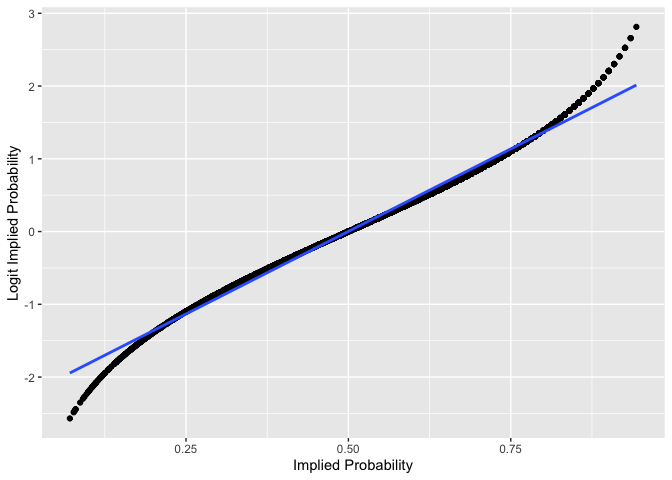
Visualize the relationship between the Implied Probabilities of the odds in original and transformed space. The graph also gives a sense of the distribution of the Implied Probabilities and the number of them which start racing towards to edges of transformed space (i.e. distortions close to the limits of the original scale).
df_for_graph %>%
  ggplot(aes(x=implied_prob, y=logit_prob))+
  geom_point()+
  geom_smooth(se = F, method = "lm")+
  ylab("Logit Implied Probability")+
  xlab("Implied Probability")
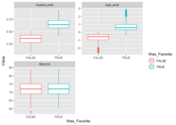
Create function to visualize data as boxplots.
boxplot_df_for_graph = function(df = df_for_graph, grouping = "Was_Favorite") {
  df$Grouping = df[,which(colnames(df) == grouping)]

  df %>%
    gather(key = "Metric", value = "Value", REACH:logit_prob) %>%
    ggplot(aes(x=Grouping, y=Value, group = Grouping, color = Grouping))+
    geom_boxplot()+
    labs(color = grouping) +
    xlab(grouping)+
    facet_wrap(.~Metric, scales = "free", nrow = 2) -> gg
  print(gg)

}
Examine distribution of predictors as a function of which fighter was the favorite.
boxplot_df_for_graph()
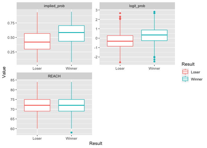
Examine distribution of predictors as a function of who won.
boxplot_df_for_graph(grouping = "Result")
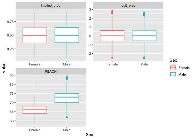
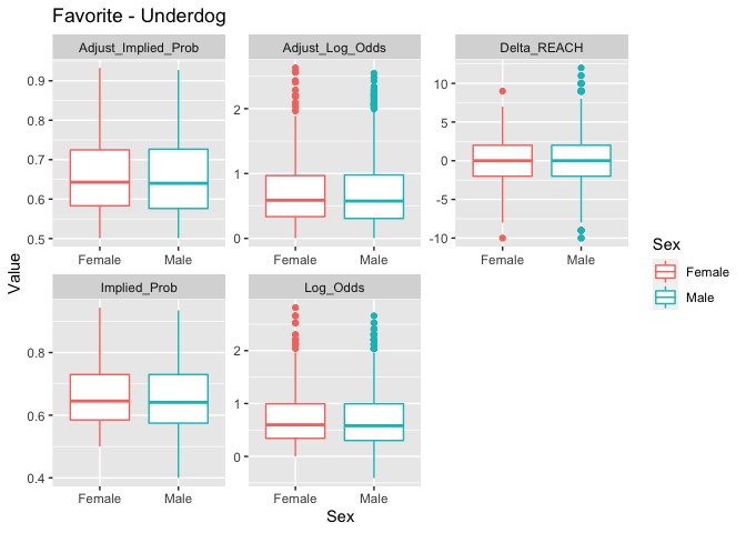
Examine distribution of predictors as a function of Sex.
boxplot_df_for_graph(grouping = "Sex")
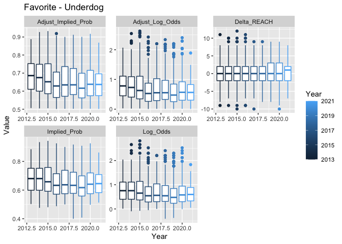
Examine distribution of predictors as a function of Year.
boxplot_df_for_graph(grouping = "Year")
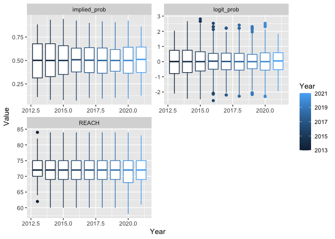
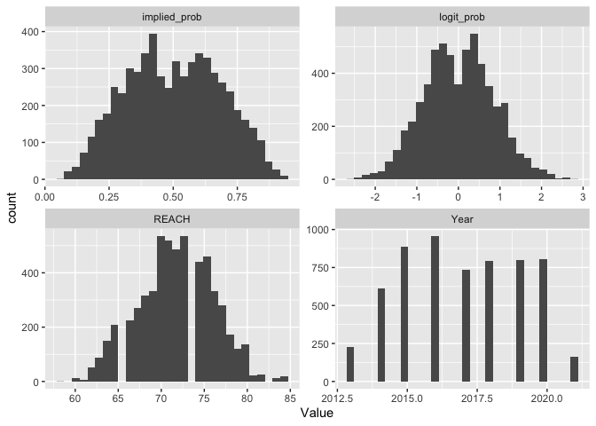
Examine distribution of potential predictors. Of course, the distributions of Implied Probabilities are missing their peaks due to the removal of fights with equal odds.
Otherwise, Reach is somewhat normally distributed.
df_for_graph %>%
  gather(key = "Metric", value = "Value", Year:logit_prob) %>%
  ggplot(aes(x=Value))+
  geom_histogram()+
  facet_wrap(.~Metric, scales = "free", nrow = 3)
Compute Differences between Fighters
Create separate data frames for favorites and underdogs, then merge them.
# Favorites
df_stats %>%
  dplyr::filter(Was_Favorite) %>%
  dplyr::select(
    fight_id
    , Sex
    , Favorite_Won
    , Year
    , REACH
    , implied_prob
    , logit_prob
    ) -> df_favs

# Underdogs
df_stats %>%
  dplyr::filter(!Was_Favorite) %>%
  dplyr::select(
    fight_id
    , Sex
    , Favorite_Won
    , Year
    , REACH
    , implied_prob
    , logit_prob
  ) -> df_under
# rename
df_under %>%
  rename(
    U_REACH = REACH
    , U_implied_prob = implied_prob
    , U_logit_prob = logit_prob
  ) -> df_under

# Merge
df_both = merge(df_under, df_favs)
Examine new dataframe.
summary(df_both)

##     fight_id        Sex       Favorite_Won         Year         U_REACH
##  1      :   1   Female: 385   Mode :logical   Min.   :2013   Min.   :58.00
##  2      :   1   Male  :2603   FALSE:1057      1st Qu.:2015   1st Qu.:69.00
##  3      :   1                 TRUE :1931      Median :2017   Median :72.00
##  4      :   1                                 Mean   :2017   Mean   :71.62
##  5      :   1                                 3rd Qu.:2019   3rd Qu.:75.00
##  6      :   1                                 Max.   :2021   Max.   :84.00
##  (Other):2982                                                NA's   :159
##  U_implied_prob     U_logit_prob          REACH        implied_prob
##  Min.   :0.07117   Min.   :-2.56879   Min.   :60.00   Min.   :0.4000
##  1st Qu.:0.27548   1st Qu.:-0.96698   1st Qu.:69.00   1st Qu.:0.5780
##  Median :0.36101   Median :-0.57098   Median :72.00   Median :0.6410
##  Mean   :0.34701   Mean   :-0.67036   Mean   :71.87   Mean   :0.6576
##  3rd Qu.:0.42553   3rd Qu.:-0.30010   3rd Qu.:75.00   3rd Qu.:0.7299
##  Max.   :0.52356   Max.   : 0.09431   Max.   :84.00   Max.   :0.9434
##                                       NA's   :54
##    logit_prob
##  Min.   :-0.4055
##  1st Qu.: 0.3147
##  Median : 0.5798
##  Mean   : 0.6948
##  3rd Qu.: 0.9943
##  Max.   : 2.8134
##
How many fights do we have?
nrow(df_both)

## [1] 2988
How often does the favorite win?
mean(df_both$Favorite_Won)

## [1] 0.6462517
Compute differences in Reach. Also, adjust for the overround.
df_both %>%
  dplyr::group_by(fight_id) %>%
  dplyr::summarise(
    Favorite_Won=Favorite_Won
    , Sex=Sex
    , Year=Year
    , Delta_REACH = REACH - U_REACH
    , Log_Odds = logit_prob
    , Implied_Prob = implied_prob
    , Adjust_Implied_Prob = implied_prob - (implied_prob + U_implied_prob - 1)/2
  ) -> df_og_diff
Get Adjusted Log Odds.
df_og_diff %>%
  mutate(Adjust_Log_Odds = qlogis(Adjust_Implied_Prob)) -> df_og_diff
Examine new dataframe. Notice that Adjusted Implied Probabilities never go under 0.5. Similarly, Adjusted Log Odds never go below 0.
summary(df_og_diff)

##     fight_id    Favorite_Won        Sex            Year       Delta_REACH
##  1      :   1   Mode :logical   Female: 385   Min.   :2013   Min.   :-10.0000
##  2      :   1   FALSE:1057      Male  :2603   1st Qu.:2015   1st Qu.: -2.0000
##  3      :   1   TRUE :1931                    Median :2017   Median :  0.0000
##  4      :   1                                 Mean   :2017   Mean   :  0.2748
##  5      :   1                                 3rd Qu.:2019   3rd Qu.:  2.0000
##  6      :   1                                 Max.   :2021   Max.   : 12.0000
##  (Other):2982                                                NA's   :211
##     Log_Odds        Implied_Prob    Adjust_Implied_Prob Adjust_Log_Odds
##  Min.   :-0.4055   Min.   :0.4000   Min.   :0.5012      Min.   :0.004782
##  1st Qu.: 0.3147   1st Qu.:0.5780   1st Qu.:0.5778      1st Qu.:0.313771
##  Median : 0.5798   Median :0.6410   Median :0.6406      Median :0.577952
##  Mean   : 0.6948   Mean   :0.6576   Mean   :0.6553      Mean   :0.682173
##  3rd Qu.: 0.9943   3rd Qu.:0.7299   3rd Qu.:0.7261      3rd Qu.:0.974797
##  Max.   : 2.8134   Max.   :0.9434   Max.   :0.9327      Max.   :2.628868
##
Examine correlations among potential predictors.
df_cor_diff = cor(df_og_diff[5:9], method = c("spearman"), use = "na.or.complete")
corrplot(df_cor_diff)
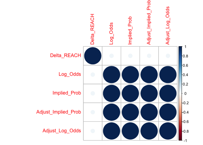
df_cor_diff

##                     Delta_REACH   Log_Odds Implied_Prob Adjust_Implied_Prob
## Delta_REACH          1.00000000 0.05662437   0.05662437          0.05569811
## Log_Odds             0.05662437 1.00000000   1.00000000          0.99449602
## Implied_Prob         0.05662437 1.00000000   1.00000000          0.99449602
## Adjust_Implied_Prob  0.05569811 0.99449602   0.99449602          1.00000000
## Adjust_Log_Odds      0.05569811 0.99449602   0.99449602          1.00000000
##                     Adjust_Log_Odds
## Delta_REACH              0.05569811
## Log_Odds                 0.99449602
## Implied_Prob             0.99449602
## Adjust_Implied_Prob      1.00000000
## Adjust_Log_Odds          1.00000000
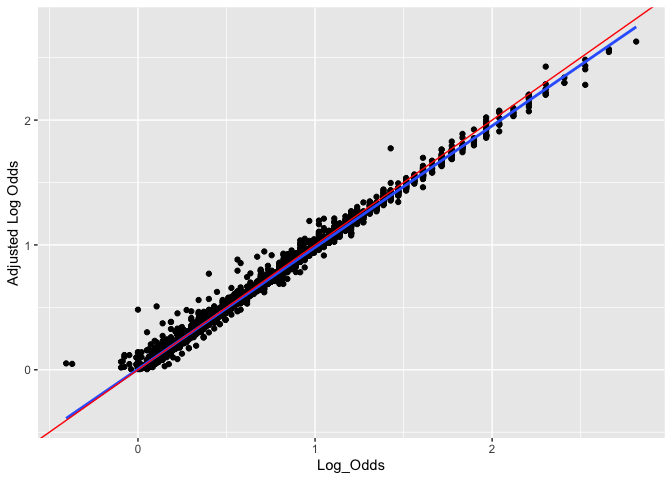
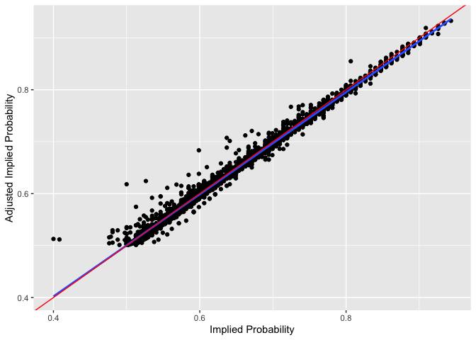
Visualize the relationship between Log Odds and Adjusted Log Odds. The red line is y=x whereas the blue line is the line of best fit.
The adjustments do not appear to vary with respect to Log Odds (i.e. closer contests did not tend to have more overround than more disperate ones, etc.).
df_og_diff %>%
  ggplot(aes(x=Log_Odds, y=Adjust_Log_Odds))+
  geom_point()+
  geom_smooth(se = F, method = "lm")+
  geom_abline(slope=1, color = "red")+
  ylab("Adjusted Log Odds")+
  xlab("Log_Odds")
Plot similar graph for Implied Probabilities.
df_og_diff %>%
  ggplot(aes(x=Implied_Prob, y=Adjust_Implied_Prob))+
  geom_point()+
  geom_smooth(se = F, method = "lm")+
  geom_abline(slope=1, color = "red")+
  ylab("Adjusted Implied Probability")+
  xlab("Implied Probability")
Deal with Missing Values
missing_reach <- round(mean(is.na(df_og_diff$Delta_REACH))*100)
How many Reach entries are missing? Around 7%.
df_og_diff %>%
  select("Delta_REACH", "fight_id") -> df_for_amelia

missmap(df_for_amelia)
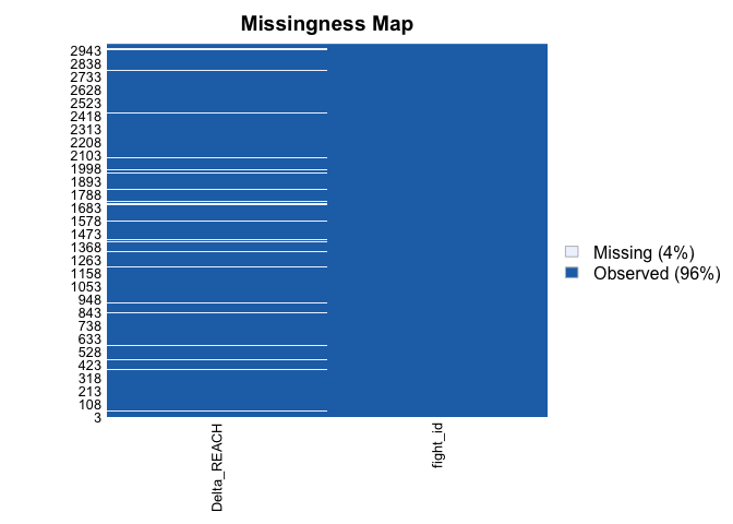
Is there a relationship between missingness of Reach and actual values of Reach? Based on the random sample below, fighters with no recorded Reach appear to not be popular overall. Therefore, they are likely NOT strong competitors on average. This will be something to keep in mind as it could introduce some kind of bias into the dataset / results.
df_master %>%
  dplyr::filter(is.na(REACH)) %>%
  dplyr::select(
  "Date"
  , "NAME"
  , "FightWeightClass"
  ) -> df_reach_nas

kable(df_reach_nas[sample(1:nrow(df_reach_nas), nrow(df_reach_nas)/10),])
| Date | NAME | FightWeightClass | |
|---|---|---|---|
| 192 | 2014-01-04 | Shunichi Shimizu | Bantamweight |
| 159 | 2014-10-04 | Niklas Backstrom | Featherweight |
| 85 | 2017-01-28 | JC Cottrell | Lightweight |
| 43 | 2017-10-28 | Christian Colombo | Heavyweight |
| 4 | 2016-05-29 | Alberto Uda | Middleweight |
| 158 | 2015-06-20 | Niklas Backstrom | Featherweight |
| 166 | 2013-11-30 | Peggy Morgan | Bantamweight |
| 27 | 2015-11-07 | Bruno Rodrigues | Bantamweight |
| 70 | 2016-04-10 | Filip Pejic | Bantamweight |
| 123 | 2016-02-21 | Kelly Faszholz | Bantamweight |
| 106 | 2016-08-06 | Joseph Gigliotti | Middleweight |
| 69 | 2016-07-08 | Fernando Bruno | Featherweight |
| 65 | 2013-12-28 | Estevan Payan | Featherweight |
| 148 | 2016-07-07 | Mehdi Baghdad | Lightweight |
| 119 | 2017-10-07 | Kalindra Faria | Flyweight |
| 214 | 2015-09-26 | Yusuke Kasuya | Lightweight |
| 39 | 2014-11-15 | Chris Heatherly | Welterweight |
| 154 | 2016-11-19 | Milana Dudieva | Bantamweight |
| 194 | 2015-08-08 | Sirwan Kakai | Bantamweight |
| 167 | 2014-01-04 | Quinn Mulhern | Lightweight |
| 5 | 2017-02-19 | Alex Ricci | Lightweight |
Compare the summaries of the subset of data without NAs to the one with NAs to identify notable differences.
df_og_diff %>%
  dplyr::filter(is.na(Delta_REACH)) -> df_nas

df_og_diff %>%
  dplyr::filter(!is.na(Delta_REACH)) -> df_nonas

summary(df_nas)

##     fight_id   Favorite_Won        Sex           Year       Delta_REACH
##  1      :  1   Mode :logical   Female: 38   Min.   :2013   Min.   : NA
##  4      :  1   FALSE:52        Male  :173   1st Qu.:2014   1st Qu.: NA
##  39     :  1   TRUE :159                    Median :2015   Median : NA
##  48     :  1                                Mean   :2015   Mean   :NaN
##  78     :  1                                3rd Qu.:2016   3rd Qu.: NA
##  90     :  1                                Max.   :2021   Max.   : NA
##  (Other):205                                               NA's   :211
##     Log_Odds         Implied_Prob    Adjust_Implied_Prob Adjust_Log_Odds
##  Min.   :-0.07696   Min.   :0.4808   Min.   :0.5064      Min.   :0.02564
##  1st Qu.: 0.37106   1st Qu.:0.5917   1st Qu.:0.5893      1st Qu.:0.36108
##  Median : 0.61619   Median :0.6494   Median :0.6504      Median :0.62073
##  Mean   : 0.73200   Mean   :0.6660   Mean   :0.6621      Mean   :0.71134
##  3rd Qu.: 1.07881   3rd Qu.:0.7463   3rd Qu.:0.7389      3rd Qu.:1.04018
##  Max.   : 2.40795   Max.   :0.9174   Max.   :0.9088      Max.   :2.29865
##

summary(df_nonas)

##     fight_id    Favorite_Won        Sex            Year       Delta_REACH
##  2      :   1   Mode :logical   Female: 347   Min.   :2013   Min.   :-10.0000
##  3      :   1   FALSE:1005      Male  :2430   1st Qu.:2015   1st Qu.: -2.0000
##  5      :   1   TRUE :1772                    Median :2017   Median :  0.0000
##  6      :   1                                 Mean   :2017   Mean   :  0.2748
##  7      :   1                                 3rd Qu.:2019   3rd Qu.:  2.0000
##  8      :   1                                 Max.   :2021   Max.   : 12.0000
##  (Other):2771
##     Log_Odds        Implied_Prob    Adjust_Implied_Prob Adjust_Log_Odds
##  Min.   :-0.4055   Min.   :0.4000   Min.   :0.5012      Min.   :0.004782
##  1st Qu.: 0.3147   1st Qu.:0.5780   1st Qu.:0.5773      1st Qu.:0.311586
##  Median : 0.5798   Median :0.6410   Median :0.6399      Median :0.574930
##  Mean   : 0.6919   Mean   :0.6570   Mean   :0.6548      Mean   :0.679957
##  3rd Qu.: 0.9676   3rd Qu.:0.7246   3rd Qu.:0.7248      3rd Qu.:0.968347
##  Max.   : 2.8134   Max.   :0.9434   Max.   :0.9327      Max.   :2.628868
##
Favorites appear to be more likely to win when Reach is NA despite not being substantially more favored (see above).
mean(df_nas$Favorite_Won) - mean(df_nonas$Favorite_Won)

## [1] 0.1154558
Using original dataset, look at if those without Reach entry tend to be favored or not. Indeed they tended to be the underdogs. Therefore, it seems like those with Reach NAs tend to underperform relative to their odds, when considering the above. As such, removing entries with missing Reach data in a future analysis could affect the results.
df_stats %>%
  dplyr::filter(is.na(REACH)) -> df_nas_odds

mean(df_nas_odds$implied_prob)

## [1] 0.4031639

mean(df_nas_odds$Was_Favorite)

## [1] 0.2535211
Also, the fights with Reach NAs are a couple years older on average. This may be due to improved stats collection and tracking through the years.
mean(df_nas$Year) - mean(df_nonas$Year)

## [1] -2.064192
I may consider a simple random imputation for the model with both Reach and Log Odds as predictors, to avoid losing cases with higher rates of underperformance.
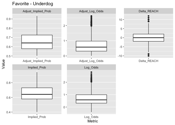
Visualize Difference Data
Create function to generate boxplots of difference data.
# function for box plot
boxplot_df_og_diff = function(df = df_og_diff, grouping = NULL, do_result = F) {

  if (is.null(grouping)) {

    if (do_result) {
      df %>%
        gather(key = "Metric", value = "Value", Delta_REACH:Adjust_Log_Odds) %>%
        dplyr::mutate(Value = ifelse(Favorite_Won, Value, -Value)) %>%  # THIS FLIPS SIGN
        ggplot(aes(x=Metric, y=Value))+
        geom_boxplot()+
        facet_wrap(.~Metric, scales = "free", nrow = 2)+
        ggtitle("Winner - Loser") -> gg
    } else {
      df %>%
        gather(key = "Metric", value = "Value", Delta_REACH:Adjust_Log_Odds) %>%
        ggplot(aes(x=Metric, y=Value))+
        geom_boxplot()+
        facet_wrap(.~Metric, scales = "free", nrow = 2)+
        ggtitle("Favorite - Underdog") -> gg
    }


  } else {

    df$Grouping = df[,which(colnames(df) == grouping)][[1]]

    df %>%
      gather(key = "Metric", value = "Value", Delta_REACH:Adjust_Log_Odds) %>%
      ggplot(aes(x=Grouping, y=Value, group = Grouping, color = Grouping))+
      geom_boxplot()+
      labs(color = grouping) +
      xlab(grouping)+
      ggtitle("Favorite - Underdog")+
      facet_wrap(.~Metric, scales = "free", nrow = 2) -> gg
  }

  print(gg)

}
Generate boxplots for potential predictors. I am including all versions of Implied Probability/Log Odds to compare them. Of course, I will only include one of these as a predictor in the model.
boxplot_df_og_diff()
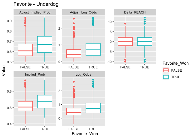
Compare predictors when the Favorite wins and loses.
boxplot_df_og_diff(grouping = "Favorite_Won")
Compare predictors as a function of Sex.
boxplot_df_og_diff(grouping = "Sex")
Compare predictors as a function of Year.
boxplot_df_og_diff(grouping = "Year")
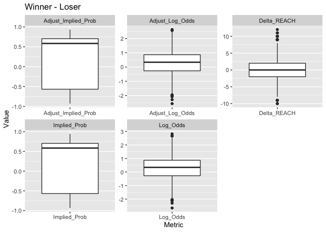
Modify predictors to look at difference in stats between Winner and Loser (instead of Favorite and Underdog).
boxplot_df_og_diff(do_result = T)
Relationship between Predictors and Outcome
Create function to plot Outcome as a function of Predictors.
# function
plot_against_log_odds = function(df = df_og_diff, variable = "Log_Odds", pred_log_odds = F, num_bin = 20, min_bin_size = 30) {

  # create dummy variable for function
  df$Dummy = df[
    ,which(colnames(df) == sprintf("%s", variable))
  ][[1]]

  # as numeric
  df$Dummy = as.numeric(df$Dummy)

  # get bins
  df$Dummy_Bin = cut(df$Dummy, num_bin)


  # get log odds of Favorite victory by bin
  df %>%
    dplyr::group_by(Dummy_Bin) %>%
    dplyr::summarise(
      Prop_of_Victory = mean(Favorite_Won)
      , Log_Odds_Victory = logit(Prop_of_Victory)
      , Size_of_Bin = length(Favorite_Won)
      , Dummy = mean(Dummy)
    ) -> fav_perf

  # extract bins
  fav_labs <- as.character(fav_perf$Dummy_Bin)
  fav_bins = as.data.frame(
    cbind(
      lower = as.numeric( sub("\\((.+),.*", "\\1", fav_labs) )
      , upper = as.numeric( sub("[^,]*,([^]]*)\\]", "\\1", fav_labs) )
    )
  )
  # get value in middle of bin
  fav_bins %>% dplyr::mutate(mid_bin = (lower + upper)/2 ) -> fav_bins
  # add mid bin column
  fav_perf$Mid_Bin = fav_bins$mid_bin

  if (pred_log_odds) {
    fav_perf %>%
    dplyr::filter(Size_of_Bin >= min_bin_size) %>%
    ggplot(aes(x=Dummy, y=Log_Odds_Victory))+
    geom_point()+
    geom_smooth(se=F , method="lm")+
    geom_abline(slope = 1, color = "red")+
    # geom_smooth()+
    ylab("Log Odds that Favorite Won")+
    xlab(sprintf("Mean %s", variable))->gg
  print(gg)
  } else {
      fav_perf %>%
      dplyr::filter(Size_of_Bin >= min_bin_size) %>%
      ggplot(aes(x=Dummy, y=Log_Odds_Victory))+
      geom_point()+
      geom_smooth(se=F , method="lm")+
      # geom_smooth()+
      ylab("Log Odds that Favorite Won")+
      xlab(sprintf("Mean %s", variable))->gg
    print(gg)
  }


}
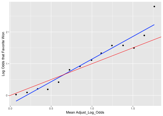
Unsurprisingly, the log odds of the implied probabilities are good linear predictors of the actual log odds of victory. Importantly, the Adjusted Log Odds appear to outperform the non-adjusted Log Odds.
plot_against_log_odds(pred_log_odds = T)
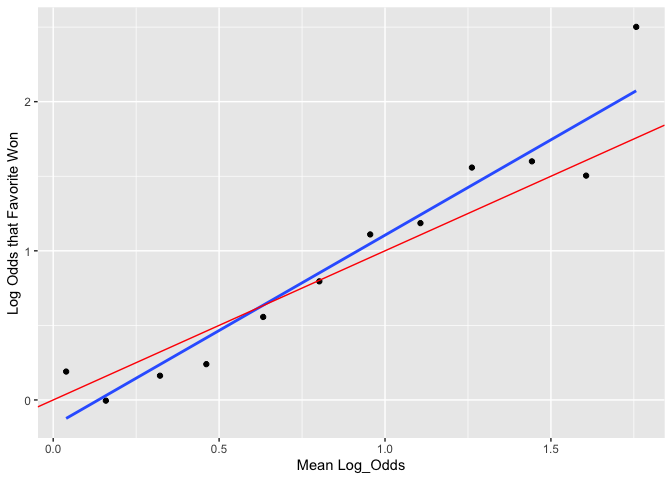
plot_against_log_odds(variable = "Adjust_Log_Odds", pred_log_odds = T)
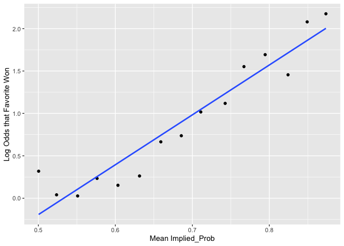
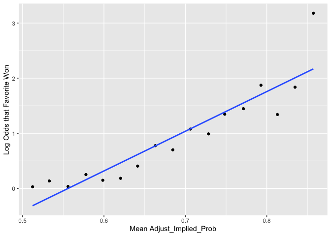
The linear fit is not quite as nice using the Implied Probability metrics. With that said, Implied Probability could likely still be used very succesfully as a predictor - the fit is still solid. Theoretically, we would have expected issues at the limits of Implied Probability (90%+). However, in practice, Implied Probabilities seldom reach those limits.
plot_against_log_odds(variable = "Implied_Prob")
plot_against_log_odds(variable = "Adjust_Implied_Prob")
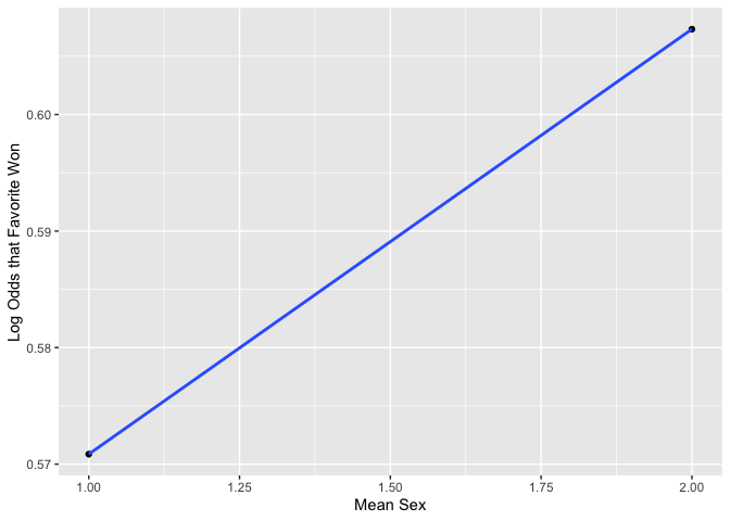
Look at y axis scale. There is virtually no difference in Log Odds of victory between sexes.
plot_against_log_odds(variable = "Sex")
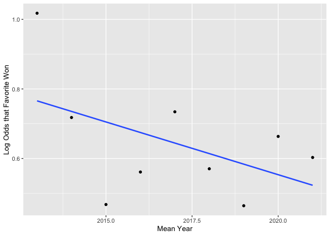
Favorites may be less likely to win in recent years. However, this may simply be an artifact of an unstable estimate for year 2013. (That point appears to have a lot of leverage.)
plot_against_log_odds(variable = "Year")
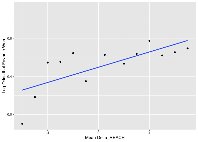
There may be a positive effect of Reach on Log Odds of victory.
plot_against_log_odds(variable = "Delta_REACH")
Assumptions
Here are the assumptions of logistic regression:
- First, binary logistic regression requires the dependent variable to be binary and ordinal logistic regression requires the dependent variable to be ordinal.
- Second, logistic regression requires the observations to be independent of each other. In other words, the observations should not come from repeated measurements or matched data.
- Third, logistic regression requires there to be little or no multicollinearity among the independent variables. This means that the independent variables should not be too highly correlated with each other.
- Fourth, logistic regression assumes linearity of independent variables and log odds. although this analysis does not require the dependent and independent variables to be related linearly, it requires that the independent variables are linearly related to the log odds.
In our case, (1) is met; (2) should be met, however, there could be random effects of Fighter or Event, etc. which likely would not impact prediction substantially but could influence explanatory analysis; (3) seems satisfactorily met (there are no major correlations); and (4) appears to be met (regardless of whether or not we use Log Odds or Implied Probability).
Adjusted Log Odds of Implied Probability as Single Predictor
fit_1 <- stan_glm(Favorite_Won ~ Adjust_Log_Odds, family=binomial(link="logit"), data = df_og_diff)

##
## SAMPLING FOR MODEL 'bernoulli' NOW (CHAIN 1).
## Chain 1:
## Chain 1: Gradient evaluation took 0.000151 seconds
## Chain 1: 1000 transitions using 10 leapfrog steps per transition would take 1.51 seconds.
## Chain 1: Adjust your expectations accordingly!
## Chain 1:
## Chain 1:
## Chain 1: Iteration:    1 / 2000 [  0%]  (Warmup)
## Chain 1: Iteration:  200 / 2000 [ 10%]  (Warmup)
## Chain 1: Iteration:  400 / 2000 [ 20%]  (Warmup)
## Chain 1: Iteration:  600 / 2000 [ 30%]  (Warmup)
## Chain 1: Iteration:  800 / 2000 [ 40%]  (Warmup)
## Chain 1: Iteration: 1000 / 2000 [ 50%]  (Warmup)
## Chain 1: Iteration: 1001 / 2000 [ 50%]  (Sampling)
## Chain 1: Iteration: 1200 / 2000 [ 60%]  (Sampling)
## Chain 1: Iteration: 1400 / 2000 [ 70%]  (Sampling)
## Chain 1: Iteration: 1600 / 2000 [ 80%]  (Sampling)
## Chain 1: Iteration: 1800 / 2000 [ 90%]  (Sampling)
## Chain 1: Iteration: 2000 / 2000 [100%]  (Sampling)
## Chain 1:
## Chain 1:  Elapsed Time: 0.607679 seconds (Warm-up)
## Chain 1:                0.709751 seconds (Sampling)
## Chain 1:                1.31743 seconds (Total)
## Chain 1:
##
## SAMPLING FOR MODEL 'bernoulli' NOW (CHAIN 2).
## Chain 2:
## Chain 2: Gradient evaluation took 0.000102 seconds
## Chain 2: 1000 transitions using 10 leapfrog steps per transition would take 1.02 seconds.
## Chain 2: Adjust your expectations accordingly!
## Chain 2:
## Chain 2:
## Chain 2: Iteration:    1 / 2000 [  0%]  (Warmup)
## Chain 2: Iteration:  200 / 2000 [ 10%]  (Warmup)
## Chain 2: Iteration:  400 / 2000 [ 20%]  (Warmup)
## Chain 2: Iteration:  600 / 2000 [ 30%]  (Warmup)
## Chain 2: Iteration:  800 / 2000 [ 40%]  (Warmup)
## Chain 2: Iteration: 1000 / 2000 [ 50%]  (Warmup)
## Chain 2: Iteration: 1001 / 2000 [ 50%]  (Sampling)
## Chain 2: Iteration: 1200 / 2000 [ 60%]  (Sampling)
## Chain 2: Iteration: 1400 / 2000 [ 70%]  (Sampling)
## Chain 2: Iteration: 1600 / 2000 [ 80%]  (Sampling)
## Chain 2: Iteration: 1800 / 2000 [ 90%]  (Sampling)
## Chain 2: Iteration: 2000 / 2000 [100%]  (Sampling)
## Chain 2:
## Chain 2:  Elapsed Time: 0.580237 seconds (Warm-up)
## Chain 2:                0.631632 seconds (Sampling)
## Chain 2:                1.21187 seconds (Total)
## Chain 2:
##
## SAMPLING FOR MODEL 'bernoulli' NOW (CHAIN 3).
## Chain 3:
## Chain 3: Gradient evaluation took 9.8e-05 seconds
## Chain 3: 1000 transitions using 10 leapfrog steps per transition would take 0.98 seconds.
## Chain 3: Adjust your expectations accordingly!
## Chain 3:
## Chain 3:
## Chain 3: Iteration:    1 / 2000 [  0%]  (Warmup)
## Chain 3: Iteration:  200 / 2000 [ 10%]  (Warmup)
## Chain 3: Iteration:  400 / 2000 [ 20%]  (Warmup)
## Chain 3: Iteration:  600 / 2000 [ 30%]  (Warmup)
## Chain 3: Iteration:  800 / 2000 [ 40%]  (Warmup)
## Chain 3: Iteration: 1000 / 2000 [ 50%]  (Warmup)
## Chain 3: Iteration: 1001 / 2000 [ 50%]  (Sampling)
## Chain 3: Iteration: 1200 / 2000 [ 60%]  (Sampling)
## Chain 3: Iteration: 1400 / 2000 [ 70%]  (Sampling)
## Chain 3: Iteration: 1600 / 2000 [ 80%]  (Sampling)
## Chain 3: Iteration: 1800 / 2000 [ 90%]  (Sampling)
## Chain 3: Iteration: 2000 / 2000 [100%]  (Sampling)
## Chain 3:
## Chain 3:  Elapsed Time: 0.582118 seconds (Warm-up)
## Chain 3:                0.678056 seconds (Sampling)
## Chain 3:                1.26017 seconds (Total)
## Chain 3:
##
## SAMPLING FOR MODEL 'bernoulli' NOW (CHAIN 4).
## Chain 4:
## Chain 4: Gradient evaluation took 9.6e-05 seconds
## Chain 4: 1000 transitions using 10 leapfrog steps per transition would take 0.96 seconds.
## Chain 4: Adjust your expectations accordingly!
## Chain 4:
## Chain 4:
## Chain 4: Iteration:    1 / 2000 [  0%]  (Warmup)
## Chain 4: Iteration:  200 / 2000 [ 10%]  (Warmup)
## Chain 4: Iteration:  400 / 2000 [ 20%]  (Warmup)
## Chain 4: Iteration:  600 / 2000 [ 30%]  (Warmup)
## Chain 4: Iteration:  800 / 2000 [ 40%]  (Warmup)
## Chain 4: Iteration: 1000 / 2000 [ 50%]  (Warmup)
## Chain 4: Iteration: 1001 / 2000 [ 50%]  (Sampling)
## Chain 4: Iteration: 1200 / 2000 [ 60%]  (Sampling)
## Chain 4: Iteration: 1400 / 2000 [ 70%]  (Sampling)
## Chain 4: Iteration: 1600 / 2000 [ 80%]  (Sampling)
## Chain 4: Iteration: 1800 / 2000 [ 90%]  (Sampling)
## Chain 4: Iteration: 2000 / 2000 [100%]  (Sampling)
## Chain 4:
## Chain 4:  Elapsed Time: 0.534413 seconds (Warm-up)
## Chain 4:                0.592038 seconds (Sampling)
## Chain 4:                1.12645 seconds (Total)
## Chain 4:

print(fit_1)

## stan_glm
##  family:       binomial [logit]
##  formula:      Favorite_Won ~ Adjust_Log_Odds
##  observations: 2988
##  predictors:   2
## ------
##                 Median MAD_SD
## (Intercept)     -0.2    0.1
## Adjust_Log_Odds  1.3    0.1
##
## ------
## * For help interpreting the printed output see ?print.stanreg
## * For info on the priors used see ?prior_summary.stanreg
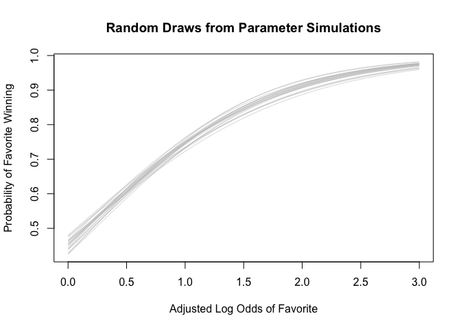
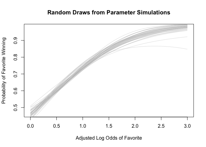
Display uncertainty in the parameters.
sims_1 <- as.matrix(fit_1)
n_sims <- nrow(sims_1)

draws_1 <- sample(n_sims, 20)

curve(invlogit(sims_1[draws_1[1],1] + sims_1[draws_1[1],2]*x)
      , from = 0
      , to = 3
      , col = "gray"
      , lwd=0.5
      , xlab="Adjusted Log Odds of Favorite"
      , ylab = "Probability of Favorite Winning"
      , main = "Random Draws from Parameter Simulations"
      )

for (j in draws_1[2:20]) {
  curve(invlogit(sims_1[j,1] + sims_1[j,2]*x)
        , col = "gray"
        , lwd=0.5
        , add=TRUE
        )
}
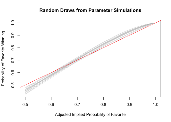
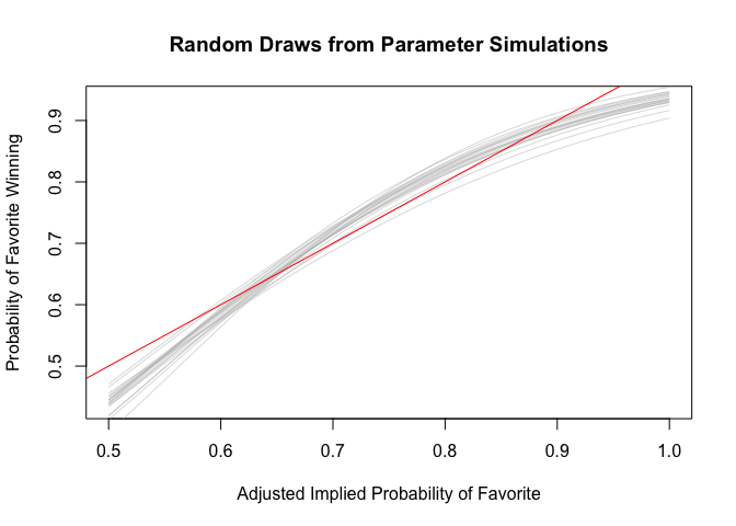
Now do the same with the backtransformed predictors (i.e. Adjusted Log Odds to Implied Probabilities). Here we can see that the negative intercept allows the model to capture the overperformance of large favorites and the underperformance of mild ones.
curve(invlogit(sims_1[draws_1[1],1] + sims_1[draws_1[1],2]*logit(x))
      , from = 0.5
      , to = 1
      , col = "gray"
      , lwd=0.5
      , xlab="Adjusted Implied Probability of Favorite"
      , ylab = "Probability of Favorite Winning"
      , main = "Random Draws from Parameter Simulations"
      )

for (j in draws_1[2:20]) {
  curve(invlogit(sims_1[j,1] + sims_1[j,2]*logit(x))
        , col = "gray"
        , lwd=0.5
        , add=TRUE
        )
}
abline(a=0, b=1, col = "red")
Evaluate intercept (i.e. with Adjusted Log Odds equal to zero). Note: Implied Probability of 50% is technically right outside the range of the data.
b1 <- fit_1$coefficients[[1]]
b2 <- fit_1$coefficients[[2]]
invlogit(0)

## [1] 0.5

invlogit(b1 + b2 * 0)

## [1] 0.4525427
Now, with Adjusted Log Odds of 1/2 which is equivalent to about 62% Adjusted Implied Probability.
invlogit(0.5)

## [1] 0.6224593

invlogit(b1 + b2 * 0.5)

## [1] 0.607421
Now, with Adjusted Log Odds of 1 which is equivalent to about 73% Adjusted Implied Probability.
invlogit(1)

## [1] 0.7310586

invlogit(b1 + b2 * 1)

## [1] 0.7433343
Now, with Adjusted Log Odds of 3/2 which is equivalent to about 82% Adjusted Implied Probability.
invlogit(3/2)

## [1] 0.8175745

invlogit(b1 + b2 * 3/2)

## [1] 0.8442581
With the intercept, the model captures the fact that mild favorites underperform whereas large favorites overperform.
Now, we’ll try the divide-by-4-rule. Indeed, the actual change in the Probability of the Favorite Winning is just under the coefficient divided by 4.
b2/4

## [1] 0.3134434

invlogit(b1 + b2 * 1) - invlogit(b1 + b2 * 0)

## [1] 0.2907916
Get point predictions using predict() and compare to Adjusted Log Odds to again get a sense of how model manages to account for underperformances and overperformances.
newx = seq(0, 3, 0.5)
new <- data.frame(Adjust_Log_Odds=newx)
pred <- predict(fit_1, type = "response", newdata = new)

new$BackTrans_Implied_Prob <- invlogit(newx)
new$Point_Pred <- pred
Get expected outcome with uncertainty.
epred <- posterior_epred(fit_1, newdata=new)

new$Means <- apply(epred, 2, mean)
new$SDs <- apply(epred, 2, sd)
Predictive distribution for new observation. Taking the mean of the predictions gives us similar results as above.
postpred <- posterior_predict(fit_1, newdata=new)

new$Mean_Pred <- apply(postpred, 2, mean)
kable(new)
| Adjust_Log_Odds | BackTrans_Implied_Prob | Point_Pred | Means | SDs | Mean_Pred |
|---|---|---|---|---|---|
| 0.0 | 0.5000000 | 0.4523726 | 0.4523726 | 0.0168735 | 0.45050 |
| 0.5 | 0.6224593 | 0.6070073 | 0.6070073 | 0.0094670 | 0.61050 |
| 1.0 | 0.7310586 | 0.7427698 | 0.7427698 | 0.0104895 | 0.73500 |
| 1.5 | 0.8175745 | 0.8434727 | 0.8434727 | 0.0125003 | 0.84300 |
| 2.0 | 0.8807971 | 0.9093447 | 0.9093447 | 0.0115072 | 0.90775 |
| 2.5 | 0.9241418 | 0.9490398 | 0.9490398 | 0.0090143 | 0.95425 |
| 3.0 | 0.9525741 | 0.9718231 | 0.9718231 | 0.0064209 | 0.97575 |
Calculate log score for pure chance.
logscore_chance <- log(0.5) * length(fit_1$fitted.values)
logscore_chance

## [1] -2071.124
Calculate log score for simply following adjusted best odds.
y <- fit_1$data$Favorite_Won
x <- fit_1$data$Adjust_Implied_Prob
logscore_bestodds <-  sum(y * log(x) + (1-y)*log(1-x))
logscore_bestodds

## [1] -1844.482
Calculate log score for model.
predp_1 <- predict(fit_1, type = "response")
logscore_1 <- sum(y * log(predp_1) + (1-y)*log(1-predp_1))
logscore_1

## [1] -1840.294
Run leave one out cross validation. There is about a two point difference between the elpd_loo estimate and the within-sample log score which makes sense since the fitted model has two parameters.
loo_1 <- loo(fit_1)
print(loo_1)

##
## Computed from 4000 by 2988 log-likelihood matrix
##
##          Estimate   SE
## elpd_loo  -1842.3 19.8
## p_loo         2.0  0.1
## looic      3684.5 39.6
## ------
## Monte Carlo SE of elpd_loo is 0.0.
##
## All Pareto k estimates are good (k < 0.5).
## See help('pareto-k-diagnostic') for details.
Adjusted Implied Probability as Single Predictor
fit_2 <- stan_glm(Favorite_Won ~ Adjust_Implied_Prob, family=binomial(link="logit"), data = df_og_diff)

##
## SAMPLING FOR MODEL 'bernoulli' NOW (CHAIN 1).
## Chain 1:
## Chain 1: Gradient evaluation took 9.6e-05 seconds
## Chain 1: 1000 transitions using 10 leapfrog steps per transition would take 0.96 seconds.
## Chain 1: Adjust your expectations accordingly!
## Chain 1:
## Chain 1:
## Chain 1: Iteration:    1 / 2000 [  0%]  (Warmup)
## Chain 1: Iteration:  200 / 2000 [ 10%]  (Warmup)
## Chain 1: Iteration:  400 / 2000 [ 20%]  (Warmup)
## Chain 1: Iteration:  600 / 2000 [ 30%]  (Warmup)
## Chain 1: Iteration:  800 / 2000 [ 40%]  (Warmup)
## Chain 1: Iteration: 1000 / 2000 [ 50%]  (Warmup)
## Chain 1: Iteration: 1001 / 2000 [ 50%]  (Sampling)
## Chain 1: Iteration: 1200 / 2000 [ 60%]  (Sampling)
## Chain 1: Iteration: 1400 / 2000 [ 70%]  (Sampling)
## Chain 1: Iteration: 1600 / 2000 [ 80%]  (Sampling)
## Chain 1: Iteration: 1800 / 2000 [ 90%]  (Sampling)
## Chain 1: Iteration: 2000 / 2000 [100%]  (Sampling)
## Chain 1:
## Chain 1:  Elapsed Time: 0.537421 seconds (Warm-up)
## Chain 1:                0.608507 seconds (Sampling)
## Chain 1:                1.14593 seconds (Total)
## Chain 1:
##
## SAMPLING FOR MODEL 'bernoulli' NOW (CHAIN 2).
## Chain 2:
## Chain 2: Gradient evaluation took 8.8e-05 seconds
## Chain 2: 1000 transitions using 10 leapfrog steps per transition would take 0.88 seconds.
## Chain 2: Adjust your expectations accordingly!
## Chain 2:
## Chain 2:
## Chain 2: Iteration:    1 / 2000 [  0%]  (Warmup)
## Chain 2: Iteration:  200 / 2000 [ 10%]  (Warmup)
## Chain 2: Iteration:  400 / 2000 [ 20%]  (Warmup)
## Chain 2: Iteration:  600 / 2000 [ 30%]  (Warmup)
## Chain 2: Iteration:  800 / 2000 [ 40%]  (Warmup)
## Chain 2: Iteration: 1000 / 2000 [ 50%]  (Warmup)
## Chain 2: Iteration: 1001 / 2000 [ 50%]  (Sampling)
## Chain 2: Iteration: 1200 / 2000 [ 60%]  (Sampling)
## Chain 2: Iteration: 1400 / 2000 [ 70%]  (Sampling)
## Chain 2: Iteration: 1600 / 2000 [ 80%]  (Sampling)
## Chain 2: Iteration: 1800 / 2000 [ 90%]  (Sampling)
## Chain 2: Iteration: 2000 / 2000 [100%]  (Sampling)
## Chain 2:
## Chain 2:  Elapsed Time: 0.492744 seconds (Warm-up)
## Chain 2:                0.591973 seconds (Sampling)
## Chain 2:                1.08472 seconds (Total)
## Chain 2:
##
## SAMPLING FOR MODEL 'bernoulli' NOW (CHAIN 3).
## Chain 3:
## Chain 3: Gradient evaluation took 9.2e-05 seconds
## Chain 3: 1000 transitions using 10 leapfrog steps per transition would take 0.92 seconds.
## Chain 3: Adjust your expectations accordingly!
## Chain 3:
## Chain 3:
## Chain 3: Iteration:    1 / 2000 [  0%]  (Warmup)
## Chain 3: Iteration:  200 / 2000 [ 10%]  (Warmup)
## Chain 3: Iteration:  400 / 2000 [ 20%]  (Warmup)
## Chain 3: Iteration:  600 / 2000 [ 30%]  (Warmup)
## Chain 3: Iteration:  800 / 2000 [ 40%]  (Warmup)
## Chain 3: Iteration: 1000 / 2000 [ 50%]  (Warmup)
## Chain 3: Iteration: 1001 / 2000 [ 50%]  (Sampling)
## Chain 3: Iteration: 1200 / 2000 [ 60%]  (Sampling)
## Chain 3: Iteration: 1400 / 2000 [ 70%]  (Sampling)
## Chain 3: Iteration: 1600 / 2000 [ 80%]  (Sampling)
## Chain 3: Iteration: 1800 / 2000 [ 90%]  (Sampling)
## Chain 3: Iteration: 2000 / 2000 [100%]  (Sampling)
## Chain 3:
## Chain 3:  Elapsed Time: 0.526684 seconds (Warm-up)
## Chain 3:                0.577734 seconds (Sampling)
## Chain 3:                1.10442 seconds (Total)
## Chain 3:
##
## SAMPLING FOR MODEL 'bernoulli' NOW (CHAIN 4).
## Chain 4:
## Chain 4: Gradient evaluation took 9.1e-05 seconds
## Chain 4: 1000 transitions using 10 leapfrog steps per transition would take 0.91 seconds.
## Chain 4: Adjust your expectations accordingly!
## Chain 4:
## Chain 4:
## Chain 4: Iteration:    1 / 2000 [  0%]  (Warmup)
## Chain 4: Iteration:  200 / 2000 [ 10%]  (Warmup)
## Chain 4: Iteration:  400 / 2000 [ 20%]  (Warmup)
## Chain 4: Iteration:  600 / 2000 [ 30%]  (Warmup)
## Chain 4: Iteration:  800 / 2000 [ 40%]  (Warmup)
## Chain 4: Iteration: 1000 / 2000 [ 50%]  (Warmup)
## Chain 4: Iteration: 1001 / 2000 [ 50%]  (Sampling)
## Chain 4: Iteration: 1200 / 2000 [ 60%]  (Sampling)
## Chain 4: Iteration: 1400 / 2000 [ 70%]  (Sampling)
## Chain 4: Iteration: 1600 / 2000 [ 80%]  (Sampling)
## Chain 4: Iteration: 1800 / 2000 [ 90%]  (Sampling)
## Chain 4: Iteration: 2000 / 2000 [100%]  (Sampling)
## Chain 4:
## Chain 4:  Elapsed Time: 0.51957 seconds (Warm-up)
## Chain 4:                0.610287 seconds (Sampling)
## Chain 4:                1.12986 seconds (Total)
## Chain 4:

print(fit_2)

## stan_glm
##  family:       binomial [logit]
##  formula:      Favorite_Won ~ Adjust_Implied_Prob
##  observations: 2988
##  predictors:   2
## ------
##                     Median MAD_SD
## (Intercept)         -3.2    0.3
## Adjust_Implied_Prob  5.9    0.4
##
## ------
## * For help interpreting the printed output see ?print.stanreg
## * For info on the priors used see ?prior_summary.stanreg
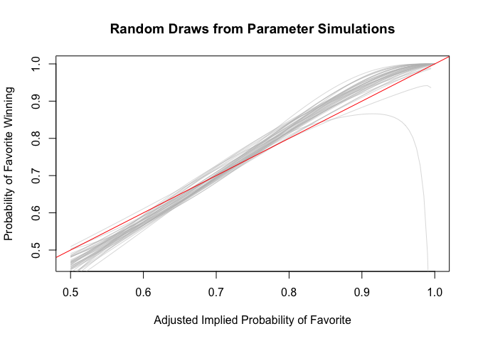
Display uncertainty in the parameters.
sims_2 <- as.matrix(fit_2)
n_sims_2 <- nrow(sims_2)

draws_2 <- sample(n_sims_2, 20)

curve(invlogit(sims_2[draws_2[1],1] + sims_2[draws_2[1],2]*x)
      , from = 0.5
      , to = 1
      , col = "gray"
      , lwd=0.5
      , xlab="Adjusted Implied Probability of Favorite"
      , ylab = "Probability of Favorite Winning"
      , main = "Random Draws from Parameter Simulations"
      )

for (j in draws_2[2:20]) {
  curve(invlogit(sims_2[j,1] + sims_2[j,2]*x)
        , col = "gray"
        , lwd=0.5
        , add=TRUE
        )
}
abline(a=0, b=1, col = "red")
Get point predictions using predict() and compare to Adjusted Implied Probabilities to get a sense of how model manages to account for underperformances and overperformances.
newx_2 = seq(0.5, 1, 0.1)
new_2 <- data.frame(Adjust_Implied_Prob=newx_2)
new_2$Point_Pred <- predict(fit_2, type = "response", newdata = new_2)
Get expected outcome with uncertainty.
epred_2 <- posterior_epred(fit_2, newdata=new_2)

new_2$Means <- apply(epred_2, 2, mean)
new_2$SDs <- apply(epred_2, 2, sd)
Predictive distribution for new observation. Taking the mean of the predictions gives us similar results as above.
postpred_2 <- posterior_predict(fit_2, newdata=new_2)

new_2$Mean_Pred <- apply(postpred_2, 2, mean)
kable(new_2)
| Adjust_Implied_Prob | Point_Pred | Means | SDs | Mean_Pred |
|---|---|---|---|---|
| 0.5 | 0.4346352 | 0.4346352 | 0.0178472 | 0.43400 |
| 0.6 | 0.5812958 | 0.5812958 | 0.0106102 | 0.57450 |
| 0.7 | 0.7148974 | 0.7148974 | 0.0100209 | 0.72175 |
| 0.8 | 0.8189411 | 0.8189411 | 0.0122480 | 0.80925 |
| 0.9 | 0.8906131 | 0.8906131 | 0.0119773 | 0.88875 |
| 1.0 | 0.9359914 | 0.9359914 | 0.0099081 | 0.93300 |
Calculate log score for second model (i.e. with Implied Probabilities). The log score is marginally worst than the one using the Adjusted Log Odds (-1840.29).
predp_2 <- predict(fit_2, type = "response")
logscore_2 <- sum(y * log(predp_2) + (1-y)*log(1-predp_2))
logscore_2

## [1] -1841.472
Run leave one out cross validation. Similarly, the elpd_loo is marginally worst than the one using the Adjusted Adjusted Log Odds (-1842.27).
loo_2 <- loo(fit_2)
print(loo_2)

##
## Computed from 4000 by 2988 log-likelihood matrix
##
##          Estimate   SE
## elpd_loo  -1843.5 19.7
## p_loo         2.0  0.1
## looic      3687.0 39.5
## ------
## Monte Carlo SE of elpd_loo is 0.0.
##
## All Pareto k estimates are good (k < 0.5).
## See help('pareto-k-diagnostic') for details.
The difference between using the Adjusted Log Odds or Implied Probabilities as a predictor is fairly small. However, using the Adjsuted Log Odds makes more sense in principle and leads to a marginally better performance. Also, it is trivially easy to back-transform the predictors for interpretability. Therefore, we will use Adjusted Log Odds.
Adjusted Log Odds with Square Term.
df_og_diff$Adjust_Log_Odds_sq = (df_og_diff$Adjust_Log_Odds)^2
fit_3 <- stan_glm(Favorite_Won ~ Adjust_Log_Odds + Adjust_Log_Odds_sq, family=binomial(link="logit"), data = df_og_diff)

##
## SAMPLING FOR MODEL 'bernoulli' NOW (CHAIN 1).
## Chain 1:
## Chain 1: Gradient evaluation took 9.6e-05 seconds
## Chain 1: 1000 transitions using 10 leapfrog steps per transition would take 0.96 seconds.
## Chain 1: Adjust your expectations accordingly!
## Chain 1:
## Chain 1:
## Chain 1: Iteration:    1 / 2000 [  0%]  (Warmup)
## Chain 1: Iteration:  200 / 2000 [ 10%]  (Warmup)
## Chain 1: Iteration:  400 / 2000 [ 20%]  (Warmup)
## Chain 1: Iteration:  600 / 2000 [ 30%]  (Warmup)
## Chain 1: Iteration:  800 / 2000 [ 40%]  (Warmup)
## Chain 1: Iteration: 1000 / 2000 [ 50%]  (Warmup)
## Chain 1: Iteration: 1001 / 2000 [ 50%]  (Sampling)
## Chain 1: Iteration: 1200 / 2000 [ 60%]  (Sampling)
## Chain 1: Iteration: 1400 / 2000 [ 70%]  (Sampling)
## Chain 1: Iteration: 1600 / 2000 [ 80%]  (Sampling)
## Chain 1: Iteration: 1800 / 2000 [ 90%]  (Sampling)
## Chain 1: Iteration: 2000 / 2000 [100%]  (Sampling)
## Chain 1:
## Chain 1:  Elapsed Time: 1.46779 seconds (Warm-up)
## Chain 1:                1.4207 seconds (Sampling)
## Chain 1:                2.88849 seconds (Total)
## Chain 1:
##
## SAMPLING FOR MODEL 'bernoulli' NOW (CHAIN 2).
## Chain 2:
## Chain 2: Gradient evaluation took 9.6e-05 seconds
## Chain 2: 1000 transitions using 10 leapfrog steps per transition would take 0.96 seconds.
## Chain 2: Adjust your expectations accordingly!
## Chain 2:
## Chain 2:
## Chain 2: Iteration:    1 / 2000 [  0%]  (Warmup)
## Chain 2: Iteration:  200 / 2000 [ 10%]  (Warmup)
## Chain 2: Iteration:  400 / 2000 [ 20%]  (Warmup)
## Chain 2: Iteration:  600 / 2000 [ 30%]  (Warmup)
## Chain 2: Iteration:  800 / 2000 [ 40%]  (Warmup)
## Chain 2: Iteration: 1000 / 2000 [ 50%]  (Warmup)
## Chain 2: Iteration: 1001 / 2000 [ 50%]  (Sampling)
## Chain 2: Iteration: 1200 / 2000 [ 60%]  (Sampling)
## Chain 2: Iteration: 1400 / 2000 [ 70%]  (Sampling)
## Chain 2: Iteration: 1600 / 2000 [ 80%]  (Sampling)
## Chain 2: Iteration: 1800 / 2000 [ 90%]  (Sampling)
## Chain 2: Iteration: 2000 / 2000 [100%]  (Sampling)
## Chain 2:
## Chain 2:  Elapsed Time: 1.3878 seconds (Warm-up)
## Chain 2:                1.53574 seconds (Sampling)
## Chain 2:                2.92354 seconds (Total)
## Chain 2:
##
## SAMPLING FOR MODEL 'bernoulli' NOW (CHAIN 3).
## Chain 3:
## Chain 3: Gradient evaluation took 9.4e-05 seconds
## Chain 3: 1000 transitions using 10 leapfrog steps per transition would take 0.94 seconds.
## Chain 3: Adjust your expectations accordingly!
## Chain 3:
## Chain 3:
## Chain 3: Iteration:    1 / 2000 [  0%]  (Warmup)
## Chain 3: Iteration:  200 / 2000 [ 10%]  (Warmup)
## Chain 3: Iteration:  400 / 2000 [ 20%]  (Warmup)
## Chain 3: Iteration:  600 / 2000 [ 30%]  (Warmup)
## Chain 3: Iteration:  800 / 2000 [ 40%]  (Warmup)
## Chain 3: Iteration: 1000 / 2000 [ 50%]  (Warmup)
## Chain 3: Iteration: 1001 / 2000 [ 50%]  (Sampling)
## Chain 3: Iteration: 1200 / 2000 [ 60%]  (Sampling)
## Chain 3: Iteration: 1400 / 2000 [ 70%]  (Sampling)
## Chain 3: Iteration: 1600 / 2000 [ 80%]  (Sampling)
## Chain 3: Iteration: 1800 / 2000 [ 90%]  (Sampling)
## Chain 3: Iteration: 2000 / 2000 [100%]  (Sampling)
## Chain 3:
## Chain 3:  Elapsed Time: 1.48475 seconds (Warm-up)
## Chain 3:                1.52879 seconds (Sampling)
## Chain 3:                3.01354 seconds (Total)
## Chain 3:
##
## SAMPLING FOR MODEL 'bernoulli' NOW (CHAIN 4).
## Chain 4:
## Chain 4: Gradient evaluation took 9.9e-05 seconds
## Chain 4: 1000 transitions using 10 leapfrog steps per transition would take 0.99 seconds.
## Chain 4: Adjust your expectations accordingly!
## Chain 4:
## Chain 4:
## Chain 4: Iteration:    1 / 2000 [  0%]  (Warmup)
## Chain 4: Iteration:  200 / 2000 [ 10%]  (Warmup)
## Chain 4: Iteration:  400 / 2000 [ 20%]  (Warmup)
## Chain 4: Iteration:  600 / 2000 [ 30%]  (Warmup)
## Chain 4: Iteration:  800 / 2000 [ 40%]  (Warmup)
## Chain 4: Iteration: 1000 / 2000 [ 50%]  (Warmup)
## Chain 4: Iteration: 1001 / 2000 [ 50%]  (Sampling)
## Chain 4: Iteration: 1200 / 2000 [ 60%]  (Sampling)
## Chain 4: Iteration: 1400 / 2000 [ 70%]  (Sampling)
## Chain 4: Iteration: 1600 / 2000 [ 80%]  (Sampling)
## Chain 4: Iteration: 1800 / 2000 [ 90%]  (Sampling)
## Chain 4: Iteration: 2000 / 2000 [100%]  (Sampling)
## Chain 4:
## Chain 4:  Elapsed Time: 1.42941 seconds (Warm-up)
## Chain 4:                1.57456 seconds (Sampling)
## Chain 4:                3.00396 seconds (Total)
## Chain 4:

print(fit_3)

## stan_glm
##  family:       binomial [logit]
##  formula:      Favorite_Won ~ Adjust_Log_Odds + Adjust_Log_Odds_sq
##  observations: 2988
##  predictors:   3
## ------
##                    Median MAD_SD
## (Intercept)        -0.2    0.1
## Adjust_Log_Odds     1.1    0.3
## Adjust_Log_Odds_sq  0.1    0.2
##
## ------
## * For help interpreting the printed output see ?print.stanreg
## * For info on the priors used see ?prior_summary.stanreg
Display uncertainty in the parameters. Take 40 draws to capture strange behavior of some of the draws on implied probability scale.
sims_3 <- as.matrix(fit_3)
n_sims_3 <- nrow(sims_3)

draws_3 <- sample(n_sims_3, 40)

curve(invlogit(sims_3[draws_3[1],1] + sims_3[draws_3[1],2]*x + sims_3[draws_3[1],3]*(x^2))
      , from = 0
      , to = 3
      , col = "gray"
      , lwd=0.5
      , xlab="Adjusted Log Odds of Favorite"
      , ylab = "Probability of Favorite Winning"
      , main = "Random Draws from Parameter Simulations"
      )

for (j in draws_3[2:40]) {
  curve(invlogit(sims_3[j,1] + sims_3[j,2]*x + sims_3[j,3]*(x^2))
        , col = "gray"
        , lwd=0.5
        , add=TRUE
        )
}
Now do the same with the backtransformed predictors (i.e. Adjusted Log Odds to Implied Probabilities). Some of the draws exhibit strange behavior toward the limit of the implied probabilities (i.e. close to 1) whereby they dip dramatically towards lower outcome values.
curve(invlogit(sims_3[draws_3[1],1] + sims_3[draws_3[1],2]*logit(x) + sims_3[draws_3[1],3]*(logit(x)^2))
      , from = 0.5
      , to = 1
      , col = "gray"
      , lwd=0.5
      , xlab="Adjusted Implied Probability of Favorite"
      , ylab = "Probability of Favorite Winning"
      , main = "Random Draws from Parameter Simulations"
      )

for (j in draws_3[2:40]) {
  curve(invlogit(sims_3[j,1] + sims_3[j,2]*logit(x) + sims_3[j,3]*(logit(x)^2))
        , col = "gray"
        , lwd=0.5
        , add=TRUE
        )
}

abline(a=0, b=1, col = "red")
Run leave one out cross validation. The model with the square terms performs about as well as the model with the Adjusted Implied Probabilities. Therefore, we will stick with the basic single predictor model using Adjusted Log Odds as a predictor.
loo_3 <- loo(fit_3)
print(loo_3)

##
## Computed from 4000 by 2988 log-likelihood matrix
##
##          Estimate   SE
## elpd_loo  -1843.6 19.9
## p_loo         3.5  0.4
## looic      3687.1 39.9
## ------
## Monte Carlo SE of elpd_loo is 0.0.
##
## All Pareto k estimates are good (k < 0.5).
## See help('pareto-k-diagnostic') for details.
Reach as Lone Predictor
We run the model with just Reach as a predictor. There are missing Reach values that we have not replaced. Indeed, the number of observations is reduced compared to the models above.
fit_4 <- stan_glm(Favorite_Won ~ Delta_REACH, family=binomial(link="logit"), data = df_og_diff)

##
## SAMPLING FOR MODEL 'bernoulli' NOW (CHAIN 1).
## Chain 1:
## Chain 1: Gradient evaluation took 8.6e-05 seconds
## Chain 1: 1000 transitions using 10 leapfrog steps per transition would take 0.86 seconds.
## Chain 1: Adjust your expectations accordingly!
## Chain 1:
## Chain 1:
## Chain 1: Iteration:    1 / 2000 [  0%]  (Warmup)
## Chain 1: Iteration:  200 / 2000 [ 10%]  (Warmup)
## Chain 1: Iteration:  400 / 2000 [ 20%]  (Warmup)
## Chain 1: Iteration:  600 / 2000 [ 30%]  (Warmup)
## Chain 1: Iteration:  800 / 2000 [ 40%]  (Warmup)
## Chain 1: Iteration: 1000 / 2000 [ 50%]  (Warmup)
## Chain 1: Iteration: 1001 / 2000 [ 50%]  (Sampling)
## Chain 1: Iteration: 1200 / 2000 [ 60%]  (Sampling)
## Chain 1: Iteration: 1400 / 2000 [ 70%]  (Sampling)
## Chain 1: Iteration: 1600 / 2000 [ 80%]  (Sampling)
## Chain 1: Iteration: 1800 / 2000 [ 90%]  (Sampling)
## Chain 1: Iteration: 2000 / 2000 [100%]  (Sampling)
## Chain 1:
## Chain 1:  Elapsed Time: 0.470981 seconds (Warm-up)
## Chain 1:                0.51835 seconds (Sampling)
## Chain 1:                0.989331 seconds (Total)
## Chain 1:
##
## SAMPLING FOR MODEL 'bernoulli' NOW (CHAIN 2).
## Chain 2:
## Chain 2: Gradient evaluation took 8.9e-05 seconds
## Chain 2: 1000 transitions using 10 leapfrog steps per transition would take 0.89 seconds.
## Chain 2: Adjust your expectations accordingly!
## Chain 2:
## Chain 2:
## Chain 2: Iteration:    1 / 2000 [  0%]  (Warmup)
## Chain 2: Iteration:  200 / 2000 [ 10%]  (Warmup)
## Chain 2: Iteration:  400 / 2000 [ 20%]  (Warmup)
## Chain 2: Iteration:  600 / 2000 [ 30%]  (Warmup)
## Chain 2: Iteration:  800 / 2000 [ 40%]  (Warmup)
## Chain 2: Iteration: 1000 / 2000 [ 50%]  (Warmup)
## Chain 2: Iteration: 1001 / 2000 [ 50%]  (Sampling)
## Chain 2: Iteration: 1200 / 2000 [ 60%]  (Sampling)
## Chain 2: Iteration: 1400 / 2000 [ 70%]  (Sampling)
## Chain 2: Iteration: 1600 / 2000 [ 80%]  (Sampling)
## Chain 2: Iteration: 1800 / 2000 [ 90%]  (Sampling)
## Chain 2: Iteration: 2000 / 2000 [100%]  (Sampling)
## Chain 2:
## Chain 2:  Elapsed Time: 0.459119 seconds (Warm-up)
## Chain 2:                0.506495 seconds (Sampling)
## Chain 2:                0.965614 seconds (Total)
## Chain 2:
##
## SAMPLING FOR MODEL 'bernoulli' NOW (CHAIN 3).
## Chain 3:
## Chain 3: Gradient evaluation took 8.4e-05 seconds
## Chain 3: 1000 transitions using 10 leapfrog steps per transition would take 0.84 seconds.
## Chain 3: Adjust your expectations accordingly!
## Chain 3:
## Chain 3:
## Chain 3: Iteration:    1 / 2000 [  0%]  (Warmup)
## Chain 3: Iteration:  200 / 2000 [ 10%]  (Warmup)
## Chain 3: Iteration:  400 / 2000 [ 20%]  (Warmup)
## Chain 3: Iteration:  600 / 2000 [ 30%]  (Warmup)
## Chain 3: Iteration:  800 / 2000 [ 40%]  (Warmup)
## Chain 3: Iteration: 1000 / 2000 [ 50%]  (Warmup)
## Chain 3: Iteration: 1001 / 2000 [ 50%]  (Sampling)
## Chain 3: Iteration: 1200 / 2000 [ 60%]  (Sampling)
## Chain 3: Iteration: 1400 / 2000 [ 70%]  (Sampling)
## Chain 3: Iteration: 1600 / 2000 [ 80%]  (Sampling)
## Chain 3: Iteration: 1800 / 2000 [ 90%]  (Sampling)
## Chain 3: Iteration: 2000 / 2000 [100%]  (Sampling)
## Chain 3:
## Chain 3:  Elapsed Time: 0.458516 seconds (Warm-up)
## Chain 3:                0.478289 seconds (Sampling)
## Chain 3:                0.936805 seconds (Total)
## Chain 3:
##
## SAMPLING FOR MODEL 'bernoulli' NOW (CHAIN 4).
## Chain 4:
## Chain 4: Gradient evaluation took 9.1e-05 seconds
## Chain 4: 1000 transitions using 10 leapfrog steps per transition would take 0.91 seconds.
## Chain 4: Adjust your expectations accordingly!
## Chain 4:
## Chain 4:
## Chain 4: Iteration:    1 / 2000 [  0%]  (Warmup)
## Chain 4: Iteration:  200 / 2000 [ 10%]  (Warmup)
## Chain 4: Iteration:  400 / 2000 [ 20%]  (Warmup)
## Chain 4: Iteration:  600 / 2000 [ 30%]  (Warmup)
## Chain 4: Iteration:  800 / 2000 [ 40%]  (Warmup)
## Chain 4: Iteration: 1000 / 2000 [ 50%]  (Warmup)
## Chain 4: Iteration: 1001 / 2000 [ 50%]  (Sampling)
## Chain 4: Iteration: 1200 / 2000 [ 60%]  (Sampling)
## Chain 4: Iteration: 1400 / 2000 [ 70%]  (Sampling)
## Chain 4: Iteration: 1600 / 2000 [ 80%]  (Sampling)
## Chain 4: Iteration: 1800 / 2000 [ 90%]  (Sampling)
## Chain 4: Iteration: 2000 / 2000 [100%]  (Sampling)
## Chain 4:
## Chain 4:  Elapsed Time: 0.4651 seconds (Warm-up)
## Chain 4:                0.484291 seconds (Sampling)
## Chain 4:                0.949391 seconds (Total)
## Chain 4:

print(fit_4)

## stan_glm
##  family:       binomial [logit]
##  formula:      Favorite_Won ~ Delta_REACH
##  observations: 2777
##  predictors:   2
## ------
##             Median MAD_SD
## (Intercept) 0.6    0.0
## Delta_REACH 0.0    0.0
##
## ------
## * For help interpreting the printed output see ?print.stanreg
## * For info on the priors used see ?prior_summary.stanreg
Need to see additional decimal places for coefficients and SEs. It looks like there is a positive effect of Reach such that fighters with longer reaches than their opponents have a greater probability of victory than those with shorter reaches than their opponents.
fit_4$coefficients

## (Intercept) Delta_REACH
##  0.56153475  0.03062914

fit_4$ses

## (Intercept) Delta_REACH
##  0.03856440  0.01229028
Display uncertainty in the parameters. The below graphs gives a sense of the uncertainty as well as the magnitude of the effect. The effect of Reach absent any other information does appear to be positive.
sims_4 <- as.matrix(fit_4)
n_sims_4 <- nrow(sims_4)


draws_4 <- sample(n_sims_4, 20)

curve(invlogit(sims_4[draws_4[1],1] + sims_4[draws_4[1],2]*x)
      , from = -15
      , to = 15
      , col = "gray"
      , lwd=0.5
      , xlab="Difference in Reach (Favorite - Underdog; inches)"
      , ylab = "Probability of Favorite Winning"
      , main = "Random Draws from Parameter Simulations"
      )

for (j in draws_4[2:20]) {
  curve(invlogit(sims_4[j,1] + sims_4[j,2]*x)
        , col = "gray"
        , lwd=0.5
        , add=TRUE
        )
}
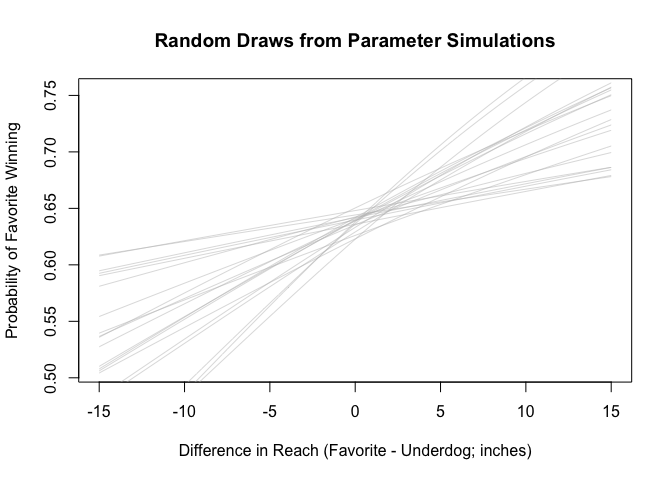
Evaluate intercept (i.e. with Difference in Reach equal to zero). This should approximately represent the average Probability of Victory of the favorite, although not exactly since Favorites have slightly greater reaches than their opponents on average (a little over a quarter inch).
b1_4 <- fit_4$coefficients[[1]]
b2_4 <- fit_4$coefficients[[2]]
invlogit(b1_4 + b2_4 * 0)

## [1] 0.6368076

mean(fit_4$data$Delta_REACH, na.rm = T)

## [1] 0.2747569
Now, we’ll try the divide by 4 rule for reach differences ranging from 1 to 5 inches.
b2_4/4 * c(1:5)

## [1] 0.007657285 0.015314570 0.022971854 0.030629139 0.038286424

b2_4_5 <- round(b2_4/4 * 5 * 100)
b2_4_1 <- round(b2_4/4 * 1 * 100, 1)
It looks like those with a 5 inch reach advantage may have about a 4% greater probability of victory than those with no reach advantage. Indeed, each one inch reach advantage corresponds to approximately a 0.8% increase in probability of victory.
Get point predictions using predict(). As with the divide-by-4-rule, a 5 inch Reach advantage is associated with almost a 4% increase with the Probability of the Favorite Winning.
newx_4 = seq(-10, 10, 1)
new_4 <- data.frame(Delta_REACH=newx_4)
new_4$Point_Pred <- predict(fit_4, type = "response", newdata = new_4)

min_point_pred <- round(min(new_4$Point_Pred)*100)
max_point_pred <- round(max(new_4$Point_Pred)*100)
diff_point_pred <- max_point_pred - min_point_pred
With the most extreme comparison, from -10 Reach to +10 Difference in Reach, the Probability of Victory jumps from around 56% to 70% - that’s a 14% difference. However, as we could see from the parameter draws, there is likely a lot of uncertainty about those more extreme estimates.
Get expected outcome with uncertainty. The uncertainty in the estimate increases with larger Reach Difference values, which was expected. However, for Reach Difference within 5 inches, the SDs for Probability of Victory are below 2%.
epred_4 <- posterior_epred(fit_4, newdata=new_4)
new_4$Means <- apply(epred_4, 2, mean)
new_4$SDs <- apply(epred_4, 2, sd)
Predictive distribution for new observation. Taking the mean of the predictions gives us similar results as above.
postpred_4 <- posterior_predict(fit_4, newdata=new_4)
new_4$Mean_Pred <- apply(postpred_4, 2, mean)
kable(new_4)
| Delta_REACH | Point_Pred | Means | SDs | Mean_Pred |
|---|---|---|---|---|
| -10 | 0.5625262 | 0.5625262 | 0.0321655 | 0.56400 |
| -9 | 0.5701204 | 0.5701204 | 0.0292140 | 0.57350 |
| -8 | 0.5776871 | 0.5776871 | 0.0263011 | 0.58275 |
| -7 | 0.5852210 | 0.5852210 | 0.0234433 | 0.57700 |
| -6 | 0.5927171 | 0.5927171 | 0.0206623 | 0.59700 |
| -5 | 0.6001704 | 0.6001704 | 0.0179895 | 0.59175 |
| -4 | 0.6075762 | 0.6075762 | 0.0154719 | 0.60250 |
| -3 | 0.6149296 | 0.6149296 | 0.0131836 | 0.61700 |
| -2 | 0.6222262 | 0.6222262 | 0.0112430 | 0.62250 |
| -1 | 0.6294616 | 0.6294616 | 0.0098272 | 0.62050 |
| 0 | 0.6366315 | 0.6366315 | 0.0091447 | 0.62875 |
| 1 | 0.6437321 | 0.6437321 | 0.0093161 | 0.63800 |
| 2 | 0.6507594 | 0.6507594 | 0.0102582 | 0.64225 |
| 3 | 0.6577100 | 0.6577100 | 0.0117494 | 0.65525 |
| 4 | 0.6645804 | 0.6645804 | 0.0135759 | 0.66275 |
| 5 | 0.6713676 | 0.6713676 | 0.0155891 | 0.66475 |
| 6 | 0.6780687 | 0.6780687 | 0.0176971 | 0.68675 |
| 7 | 0.6846809 | 0.6846809 | 0.0198441 | 0.67525 |
| 8 | 0.6912019 | 0.6912019 | 0.0219955 | 0.69250 |
| 9 | 0.6976294 | 0.6976294 | 0.0241289 | 0.69825 |
| 10 | 0.7039615 | 0.7039615 | 0.0262296 | 0.70975 |
Calculate log score for pure chance.
logscore_chance_4 <- log(0.5) * length(fit_4$fitted.values)
logscore_chance_4

## [1] -1924.87
Calculate log score for model. The simple model with Reach clearly outperforms chance.
y_4 <- fit_4$model$Favorite_Won
predp_4 <- predict(fit_4, type = "response")
logscore_4 <- sum(y_4 * log(predp_4) + (1-y_4)*log(1-predp_4))
logscore_4

## [1] -1814.43
However, does the model outperform picking the favorite at the base rate of victory (i.e. intercept only)?
base_rate_4 <- mean(fit_4$model$Favorite_Won)
logscore_inter_4 <- sum(y_4 * log(base_rate_4) + (1-y_4)*log(1-base_rate_4))
logscore_inter_4

## [1] -1817.558

score_diff_inter_4 <- round(logscore_4 - logscore_inter_4,2)
It does, but not by much - only by a logscore of 3.13, which means adding Reach as a factor probably minimally improves the predictions.
Run leave one out cross validation. We don’t have another model to compare it to but we can see that elpd_loo is is about two points more negative than the logscore calculation which is not surprising given that the model has two parameters.
loo_4 <- loo(fit_4)
print(loo_4)

##
## Computed from 4000 by 2777 log-likelihood matrix
##
##          Estimate   SE
## elpd_loo  -1816.4 14.6
## p_loo         2.0  0.0
## looic      3632.8 29.2
## ------
## Monte Carlo SE of elpd_loo is 0.0.
##
## All Pareto k estimates are good (k < 0.5).
## See help('pareto-k-diagnostic') for details.
Impute Missing Reach Values for Two Predictor Model
Do simple random imputation.
We want to avoid removing cases with missing Reach values since, as we saw earlier, those cases overrepresent underperformances and underdogs. Therefore, if we were to remove them, we may bias the results and affect the relationship between Adjusted Fight Odds and the outcome variable (Probability of Favorite Winning).
NOTE: With a more complex model, with multiple predictors and missing values across them, we may consider multiple imputation.
Based on the summary below, we see that the imputed values of Difference in Reach are virtually the same as the original ones (i.e. with NAs excluded). This is as expected, especially since we only replaced approximately 7% of Reach entries (NAs).
random_imp <- function(a) {
  missing <- is.na(a)
  n_missing <- sum(missing)
  a_obs <- a[!missing]
  imputed <- a
  imputed[missing] <- sample(a_obs, n_missing)

  return(imputed)
}

df_og_diff$Delta_REACH_imp <- random_imp(df_og_diff$Delta_REACH)

summary(df_og_diff)

##     fight_id    Favorite_Won        Sex            Year       Delta_REACH
##  1      :   1   Mode :logical   Female: 385   Min.   :2013   Min.   :-10.0000
##  2      :   1   FALSE:1057      Male  :2603   1st Qu.:2015   1st Qu.: -2.0000
##  3      :   1   TRUE :1931                    Median :2017   Median :  0.0000
##  4      :   1                                 Mean   :2017   Mean   :  0.2748
##  5      :   1                                 3rd Qu.:2019   3rd Qu.:  2.0000
##  6      :   1                                 Max.   :2021   Max.   : 12.0000
##  (Other):2982                                                NA's   :211
##     Log_Odds        Implied_Prob    Adjust_Implied_Prob Adjust_Log_Odds
##  Min.   :-0.4055   Min.   :0.4000   Min.   :0.5012      Min.   :0.004782
##  1st Qu.: 0.3147   1st Qu.:0.5780   1st Qu.:0.5778      1st Qu.:0.313771
##  Median : 0.5798   Median :0.6410   Median :0.6406      Median :0.577952
##  Mean   : 0.6948   Mean   :0.6576   Mean   :0.6553      Mean   :0.682173
##  3rd Qu.: 0.9943   3rd Qu.:0.7299   3rd Qu.:0.7261      3rd Qu.:0.974797
##  Max.   : 2.8134   Max.   :0.9434   Max.   :0.9327      Max.   :2.628868
##
##  Adjust_Log_Odds_sq Delta_REACH_imp
##  Min.   :0.000023   Min.   :-10.0000
##  1st Qu.:0.098452   1st Qu.: -2.0000
##  Median :0.334029   Median :  0.0000
##  Mean   :0.699743   Mean   :  0.2734
##  3rd Qu.:0.950229   3rd Qu.:  2.0000
##  Max.   :6.910949   Max.   : 12.0000
##
Two Predictor Model: Imputed Reach and Adjusted Log Odds
fit_5 <- stan_glm(Favorite_Won ~ Adjust_Log_Odds + Delta_REACH_imp
                  , family=binomial(link="logit")
                  , data = df_og_diff
                  )

##
## SAMPLING FOR MODEL 'bernoulli' NOW (CHAIN 1).
## Chain 1:
## Chain 1: Gradient evaluation took 0.000108 seconds
## Chain 1: 1000 transitions using 10 leapfrog steps per transition would take 1.08 seconds.
## Chain 1: Adjust your expectations accordingly!
## Chain 1:
## Chain 1:
## Chain 1: Iteration:    1 / 2000 [  0%]  (Warmup)
## Chain 1: Iteration:  200 / 2000 [ 10%]  (Warmup)
## Chain 1: Iteration:  400 / 2000 [ 20%]  (Warmup)
## Chain 1: Iteration:  600 / 2000 [ 30%]  (Warmup)
## Chain 1: Iteration:  800 / 2000 [ 40%]  (Warmup)
## Chain 1: Iteration: 1000 / 2000 [ 50%]  (Warmup)
## Chain 1: Iteration: 1001 / 2000 [ 50%]  (Sampling)
## Chain 1: Iteration: 1200 / 2000 [ 60%]  (Sampling)
## Chain 1: Iteration: 1400 / 2000 [ 70%]  (Sampling)
## Chain 1: Iteration: 1600 / 2000 [ 80%]  (Sampling)
## Chain 1: Iteration: 1800 / 2000 [ 90%]  (Sampling)
## Chain 1: Iteration: 2000 / 2000 [100%]  (Sampling)
## Chain 1:
## Chain 1:  Elapsed Time: 0.618832 seconds (Warm-up)
## Chain 1:                0.706744 seconds (Sampling)
## Chain 1:                1.32558 seconds (Total)
## Chain 1:
##
## SAMPLING FOR MODEL 'bernoulli' NOW (CHAIN 2).
## Chain 2:
## Chain 2: Gradient evaluation took 0.000102 seconds
## Chain 2: 1000 transitions using 10 leapfrog steps per transition would take 1.02 seconds.
## Chain 2: Adjust your expectations accordingly!
## Chain 2:
## Chain 2:
## Chain 2: Iteration:    1 / 2000 [  0%]  (Warmup)
## Chain 2: Iteration:  200 / 2000 [ 10%]  (Warmup)
## Chain 2: Iteration:  400 / 2000 [ 20%]  (Warmup)
## Chain 2: Iteration:  600 / 2000 [ 30%]  (Warmup)
## Chain 2: Iteration:  800 / 2000 [ 40%]  (Warmup)
## Chain 2: Iteration: 1000 / 2000 [ 50%]  (Warmup)
## Chain 2: Iteration: 1001 / 2000 [ 50%]  (Sampling)
## Chain 2: Iteration: 1200 / 2000 [ 60%]  (Sampling)
## Chain 2: Iteration: 1400 / 2000 [ 70%]  (Sampling)
## Chain 2: Iteration: 1600 / 2000 [ 80%]  (Sampling)
## Chain 2: Iteration: 1800 / 2000 [ 90%]  (Sampling)
## Chain 2: Iteration: 2000 / 2000 [100%]  (Sampling)
## Chain 2:
## Chain 2:  Elapsed Time: 0.662914 seconds (Warm-up)
## Chain 2:                0.699454 seconds (Sampling)
## Chain 2:                1.36237 seconds (Total)
## Chain 2:
##
## SAMPLING FOR MODEL 'bernoulli' NOW (CHAIN 3).
## Chain 3:
## Chain 3: Gradient evaluation took 0.000103 seconds
## Chain 3: 1000 transitions using 10 leapfrog steps per transition would take 1.03 seconds.
## Chain 3: Adjust your expectations accordingly!
## Chain 3:
## Chain 3:
## Chain 3: Iteration:    1 / 2000 [  0%]  (Warmup)
## Chain 3: Iteration:  200 / 2000 [ 10%]  (Warmup)
## Chain 3: Iteration:  400 / 2000 [ 20%]  (Warmup)
## Chain 3: Iteration:  600 / 2000 [ 30%]  (Warmup)
## Chain 3: Iteration:  800 / 2000 [ 40%]  (Warmup)
## Chain 3: Iteration: 1000 / 2000 [ 50%]  (Warmup)
## Chain 3: Iteration: 1001 / 2000 [ 50%]  (Sampling)
## Chain 3: Iteration: 1200 / 2000 [ 60%]  (Sampling)
## Chain 3: Iteration: 1400 / 2000 [ 70%]  (Sampling)
## Chain 3: Iteration: 1600 / 2000 [ 80%]  (Sampling)
## Chain 3: Iteration: 1800 / 2000 [ 90%]  (Sampling)
## Chain 3: Iteration: 2000 / 2000 [100%]  (Sampling)
## Chain 3:
## Chain 3:  Elapsed Time: 0.61107 seconds (Warm-up)
## Chain 3:                0.70918 seconds (Sampling)
## Chain 3:                1.32025 seconds (Total)
## Chain 3:
##
## SAMPLING FOR MODEL 'bernoulli' NOW (CHAIN 4).
## Chain 4:
## Chain 4: Gradient evaluation took 9.4e-05 seconds
## Chain 4: 1000 transitions using 10 leapfrog steps per transition would take 0.94 seconds.
## Chain 4: Adjust your expectations accordingly!
## Chain 4:
## Chain 4:
## Chain 4: Iteration:    1 / 2000 [  0%]  (Warmup)
## Chain 4: Iteration:  200 / 2000 [ 10%]  (Warmup)
## Chain 4: Iteration:  400 / 2000 [ 20%]  (Warmup)
## Chain 4: Iteration:  600 / 2000 [ 30%]  (Warmup)
## Chain 4: Iteration:  800 / 2000 [ 40%]  (Warmup)
## Chain 4: Iteration: 1000 / 2000 [ 50%]  (Warmup)
## Chain 4: Iteration: 1001 / 2000 [ 50%]  (Sampling)
## Chain 4: Iteration: 1200 / 2000 [ 60%]  (Sampling)
## Chain 4: Iteration: 1400 / 2000 [ 70%]  (Sampling)
## Chain 4: Iteration: 1600 / 2000 [ 80%]  (Sampling)
## Chain 4: Iteration: 1800 / 2000 [ 90%]  (Sampling)
## Chain 4: Iteration: 2000 / 2000 [100%]  (Sampling)
## Chain 4:
## Chain 4:  Elapsed Time: 0.615998 seconds (Warm-up)
## Chain 4:                0.691082 seconds (Sampling)
## Chain 4:                1.30708 seconds (Total)
## Chain 4:

print(fit_5)

## stan_glm
##  family:       binomial [logit]
##  formula:      Favorite_Won ~ Adjust_Log_Odds + Delta_REACH_imp
##  observations: 2988
##  predictors:   3
## ------
##                 Median MAD_SD
## (Intercept)     -0.2    0.1
## Adjust_Log_Odds  1.2    0.1
## Delta_REACH_imp  0.0    0.0
##
## ------
## * For help interpreting the printed output see ?print.stanreg
## * For info on the priors used see ?prior_summary.stanreg
Get better sense of coefficients. Unsurprisingly, Adjusted Log Odds still has a large effect. The (imputed) Difference in Reach still seems to have an effect. The magnitude of the effect decreased a bit but the standard error stayed about the same (compared to the model with just Reach).
fit_5$coefficients

##     (Intercept) Adjust_Log_Odds Delta_REACH_imp
##     -0.19006516      1.24198698      0.02357245

fit_5$ses

##     (Intercept) Adjust_Log_Odds Delta_REACH_imp
##      0.06827189      0.09365881      0.01213586
Display uncertainty in the parameters. The graph below plots random draws from the parameter simulations for 5 values of Difference in Reach: -10 (green), -5 inches (red), 0 inches (grey), +5 inches (blue), and +10 (yellow). We see the Difference in Reach sort of just shifts the curves (and therefore the Probability of the Favorite Winning) upwards.
sims_5 <- as.matrix(fit_5)
n_sims_5 <- nrow(sims_5)

draws_5 <- sample(n_sims_5, 20)

curve(invlogit(sims_5[draws_5[1],1] + sims_5[draws_5[1],2]*x + sims_5[draws_5[1],3]*(0))
    , from = 0
    , to = 3
    , col = "black"
    , lwd=0.0       # make invisible, just used to set up plot.
    , xlab="Adjusted Log Odds of Favorite"
    , ylab = "Probability of Favorite Winning"
    , main = "Random Draws from Parameter Simulations"
    )

for (j in draws_5) {

   curve(invlogit(sims_5[j,1] + sims_5[j,2]*x + sims_5[j,3]*(-10))
        , col = "green"
        , lwd=0.3
        , add=TRUE
        )

    curve(invlogit(sims_5[j,1] + sims_5[j,2]*x + sims_5[j,3]*(-5))
        , col = "red"
        , lwd=0.3
        , add=TRUE
        )

    curve(invlogit(sims_5[j,1] + sims_5[j,2]*x + sims_5[j,3]*(0))
        , col = "black"
        , lwd=0.3
        , add=TRUE
        )

      curve(invlogit(sims_5[j,1] + sims_5[j,2]*x + sims_5[j,3]*(+5))
        , col = "blue"
        , lwd=0.3
        , add=TRUE
        )

      curve(invlogit(sims_5[j,1] + sims_5[j,2]*x + sims_5[j,3]*(+10))
        , col = "yellow"
        , lwd=0.3
        , add=TRUE
        )
}
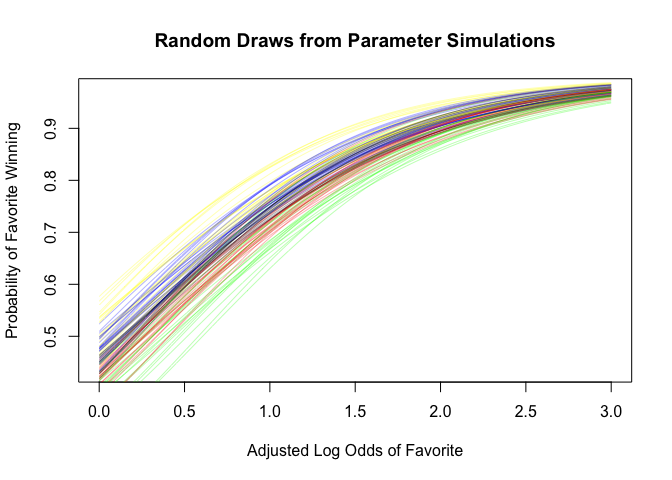
Now do the same with the backtransformed predictors (i.e. Adjusted Log Odds to Implied Probabilities). It appears that when there is no Reach Difference (i.e. black lines), the model account for some of the underperformance of mild favorites / overperformance of large favorites. Otherwise, Reach Difference simply results in a shift in the curve.
curve(invlogit(sims_5[draws_5[1],1] + sims_5[draws_5[1],2]*logit(x) + sims_5[draws_5[1],3]*(0))
    , from = 0.5
    , to = 1
    , col = "black"
    , lwd=0.0       # make invisible, just used to set up plot.
    , xlab="Adjusted Implied Probability of Favorite"
    , ylab = "Probability of Favorite Winning"
    , main = "Random Draws from Parameter Simulations"
    )

for (j in draws_5) {

   curve(invlogit(sims_5[j,1] + sims_5[j,2]*logit(x) + sims_5[j,3]*(-10))
        , col = "green"
        , lwd=0.3
        , add=TRUE
        )

    curve(invlogit(sims_5[j,1] + sims_5[j,2]*logit(x) + sims_5[j,3]*(-5))
        , col = "red"
        , lwd=0.3
        , add=TRUE
        )

    curve(invlogit(sims_5[j,1] + sims_5[j,2]*logit(x) + sims_5[j,3]*(0))
        , col = "black"
        , lwd=0.3
        , add=TRUE
        )

      curve(invlogit(sims_5[j,1] + sims_5[j,2]*logit(x) + sims_5[j,3]*(+5))
        , col = "blue"
        , lwd=0.3
        , add=TRUE
        )

      curve(invlogit(sims_5[j,1] + sims_5[j,2]*logit(x) + sims_5[j,3]*(+10))
        , col = "yellow"
        , lwd=0.3
        , add=TRUE
        )
}


abline(a=0, b=1, col = "black", lwd = 2, lty = 3)
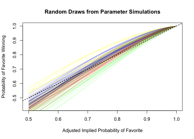
Get point predictions and compare them to Adjusted Log Odds backtransformed to Implied Probabilities.
new_5 <- data.frame(Adjust_Log_Odds=rep(newx, each = 21), Delta_REACH_imp=newx_4)
new_5$Point_Pred <- predict(fit_5, type = "response", newdata = new_5)

new_5$BackTrans_Implied_Prob <- invlogit(new_5$Adjust_Log_Odds)
Get expected outcome with uncertainty.
epred_5 <- posterior_epred(fit_5, newdata=new_5)

new_5$Means <- apply(epred_5, 2, mean)
new_5$SDs <- apply(epred_5, 2, sd)
Predictive distribution for new observation.
postpred_5 <- posterior_predict(fit_5, newdata=new_5)

new_5$Pred_Ms <- apply(postpred_5, 2, mean)
kable(new_5)
| Adjust_Log_Odds | Delta_REACH_imp | Point_Pred | BackTrans_Implied_Prob | Means | SDs | Pred_Ms |
|---|---|---|---|---|---|---|
| 0.0 | -10 | 0.3955847 | 0.5000000 | 0.3955847 | 0.0331463 | 0.38500 |
| 0.0 | -9 | 0.4011308 | 0.5000000 | 0.4011308 | 0.0308774 | 0.38350 |
| 0.0 | -8 | 0.4067158 | 0.5000000 | 0.4067158 | 0.0286508 | 0.42050 |
| 0.0 | -7 | 0.4123376 | 0.5000000 | 0.4123376 | 0.0264902 | 0.40600 |
| 0.0 | -6 | 0.4179938 | 0.5000000 | 0.4179938 | 0.0244261 | 0.42275 |
| 0.0 | -5 | 0.4236821 | 0.5000000 | 0.4236821 | 0.0224986 | 0.43050 |
| 0.0 | -4 | 0.4294000 | 0.5000000 | 0.4294000 | 0.0207595 | 0.42225 |
| 0.0 | -3 | 0.4351451 | 0.5000000 | 0.4351451 | 0.0192731 | 0.43850 |
| 0.0 | -2 | 0.4409146 | 0.5000000 | 0.4409146 | 0.0181143 | 0.43250 |
| 0.0 | -1 | 0.4467061 | 0.5000000 | 0.4467061 | 0.0173604 | 0.45100 |
| 0.0 | 0 | 0.4525167 | 0.5000000 | 0.4525167 | 0.0170750 | 0.45050 |
| 0.0 | 1 | 0.4583438 | 0.5000000 | 0.4583438 | 0.0172891 | 0.44925 |
| 0.0 | 2 | 0.4641845 | 0.5000000 | 0.4641845 | 0.0179906 | 0.46575 |
| 0.0 | 3 | 0.4700360 | 0.5000000 | 0.4700360 | 0.0191293 | 0.47025 |
| 0.0 | 4 | 0.4758956 | 0.5000000 | 0.4758956 | 0.0206345 | 0.47350 |
| 0.0 | 5 | 0.4817602 | 0.5000000 | 0.4817602 | 0.0224321 | 0.47825 |
| 0.0 | 6 | 0.4876271 | 0.5000000 | 0.4876271 | 0.0244561 | 0.48450 |
| 0.0 | 7 | 0.4934935 | 0.5000000 | 0.4934935 | 0.0266519 | 0.48300 |
| 0.0 | 8 | 0.4993563 | 0.5000000 | 0.4993563 | 0.0289766 | 0.51300 |
| 0.0 | 9 | 0.5052129 | 0.5000000 | 0.5052129 | 0.0313968 | 0.51175 |
| 0.0 | 10 | 0.5110603 | 0.5000000 | 0.5110603 | 0.0338866 | 0.49875 |
| 0.5 | -10 | 0.5486025 | 0.6224593 | 0.5486025 | 0.0317580 | 0.54125 |
| 0.5 | -9 | 0.5544326 | 0.6224593 | 0.5544326 | 0.0289347 | 0.54700 |
| 0.5 | -8 | 0.5602515 | 0.6224593 | 0.5602515 | 0.0261492 | 0.56875 |
| 0.5 | -7 | 0.5660565 | 0.6224593 | 0.5660565 | 0.0234171 | 0.56700 |
| 0.5 | -6 | 0.5718448 | 0.6224593 | 0.5718448 | 0.0207599 | 0.56750 |
| 0.5 | -5 | 0.5776135 | 0.6224593 | 0.5776135 | 0.0182088 | 0.59150 |
| 0.5 | -4 | 0.5833601 | 0.6224593 | 0.5833601 | 0.0158114 | 0.58625 |
| 0.5 | -3 | 0.5890818 | 0.6224593 | 0.5890818 | 0.0136417 | 0.59100 |
| 0.5 | -2 | 0.5947759 | 0.6224593 | 0.5947759 | 0.0118143 | 0.60325 |
| 0.5 | -1 | 0.6004400 | 0.6224593 | 0.6004400 | 0.0104937 | 0.60325 |
| 0.5 | 0 | 0.6060714 | 0.6224593 | 0.6060714 | 0.0098651 | 0.60500 |
| 0.5 | 1 | 0.6116679 | 0.6224593 | 0.6116679 | 0.0100368 | 0.61775 |
| 0.5 | 2 | 0.6172270 | 0.6224593 | 0.6172270 | 0.0109481 | 0.63375 |
| 0.5 | 3 | 0.6227465 | 0.6224593 | 0.6227465 | 0.0124154 | 0.61325 |
| 0.5 | 4 | 0.6282242 | 0.6224593 | 0.6282242 | 0.0142472 | 0.64125 |
| 0.5 | 5 | 0.6336580 | 0.6224593 | 0.6336580 | 0.0163018 | 0.63700 |
| 0.5 | 6 | 0.6390460 | 0.6224593 | 0.6390460 | 0.0184870 | 0.63600 |
| 0.5 | 7 | 0.6443862 | 0.6224593 | 0.6443862 | 0.0207450 | 0.65350 |
| 0.5 | 8 | 0.6496768 | 0.6224593 | 0.6496768 | 0.0230388 | 0.64625 |
| 0.5 | 9 | 0.6549163 | 0.6224593 | 0.6549163 | 0.0253441 | 0.64875 |
| 0.5 | 10 | 0.6601029 | 0.6224593 | 0.6601029 | 0.0276447 | 0.67225 |
| 1.0 | -10 | 0.6929719 | 0.7310586 | 0.6929719 | 0.0286974 | 0.70400 |
| 1.0 | -9 | 0.6980489 | 0.7310586 | 0.6980489 | 0.0261868 | 0.69100 |
| 1.0 | -8 | 0.7030720 | 0.7310586 | 0.7030720 | 0.0237609 | 0.70900 |
| 1.0 | -7 | 0.7080398 | 0.7310586 | 0.7080398 | 0.0214350 | 0.70825 |
| 1.0 | -6 | 0.7129508 | 0.7310586 | 0.7129508 | 0.0192294 | 0.71500 |
| 1.0 | -5 | 0.7178035 | 0.7310586 | 0.7178035 | 0.0171717 | 0.71375 |
| 1.0 | -4 | 0.7225969 | 0.7310586 | 0.7225969 | 0.0153000 | 0.71550 |
| 1.0 | -3 | 0.7273296 | 0.7310586 | 0.7273296 | 0.0136655 | 0.72325 |
| 1.0 | -2 | 0.7320006 | 0.7310586 | 0.7320006 | 0.0123344 | 0.72950 |
| 1.0 | -1 | 0.7366091 | 0.7310586 | 0.7366091 | 0.0113822 | 0.74575 |
| 1.0 | 0 | 0.7411541 | 0.7310586 | 0.7411541 | 0.0108759 | 0.73850 |
| 1.0 | 1 | 0.7456350 | 0.7310586 | 0.7456350 | 0.0108450 | 0.74275 |
| 1.0 | 2 | 0.7500511 | 0.7310586 | 0.7500511 | 0.0112620 | 0.75225 |
| 1.0 | 3 | 0.7544019 | 0.7310586 | 0.7544019 | 0.0120515 | 0.75175 |
| 1.0 | 4 | 0.7586870 | 0.7310586 | 0.7586870 | 0.0131203 | 0.76750 |
| 1.0 | 5 | 0.7629059 | 0.7310586 | 0.7629059 | 0.0143828 | 0.76125 |
| 1.0 | 6 | 0.7670586 | 0.7310586 | 0.7670586 | 0.0157720 | 0.76100 |
| 1.0 | 7 | 0.7711447 | 0.7310586 | 0.7711447 | 0.0172385 | 0.77025 |
| 1.0 | 8 | 0.7751642 | 0.7310586 | 0.7751642 | 0.0187480 | 0.78125 |
| 1.0 | 9 | 0.7791172 | 0.7310586 | 0.7791172 | 0.0202760 | 0.77825 |
| 1.0 | 10 | 0.7830037 | 0.7310586 | 0.7830037 | 0.0218057 | 0.79525 |
| 1.5 | -10 | 0.8071793 | 0.8175745 | 0.8071793 | 0.0243405 | 0.81125 |
| 1.5 | -9 | 0.8109322 | 0.8175745 | 0.8109322 | 0.0225683 | 0.79875 |
| 1.5 | -8 | 0.8146189 | 0.8175745 | 0.8146189 | 0.0209012 | 0.82650 |
| 1.5 | -7 | 0.8182394 | 0.8175745 | 0.8182394 | 0.0193490 | 0.81250 |
| 1.5 | -6 | 0.8217940 | 0.8175745 | 0.8217940 | 0.0179231 | 0.82250 |
| 1.5 | -5 | 0.8252827 | 0.8175745 | 0.8252827 | 0.0166367 | 0.82250 |
| 1.5 | -4 | 0.8287060 | 0.8175745 | 0.8287060 | 0.0155044 | 0.82800 |
| 1.5 | -3 | 0.8320641 | 0.8175745 | 0.8320641 | 0.0145417 | 0.83475 |
| 1.5 | -2 | 0.8353575 | 0.8175745 | 0.8353575 | 0.0137631 | 0.84275 |
| 1.5 | -1 | 0.8385867 | 0.8175745 | 0.8385867 | 0.0131801 | 0.83550 |
| 1.5 | 0 | 0.8417522 | 0.8175745 | 0.8417522 | 0.0127987 | 0.83950 |
| 1.5 | 1 | 0.8448545 | 0.8175745 | 0.8448545 | 0.0126172 | 0.84275 |
| 1.5 | 2 | 0.8478944 | 0.8175745 | 0.8478944 | 0.0126252 | 0.85175 |
| 1.5 | 3 | 0.8508724 | 0.8175745 | 0.8508724 | 0.0128045 | 0.85075 |
| 1.5 | 4 | 0.8537893 | 0.8175745 | 0.8537893 | 0.0131319 | 0.84950 |
| 1.5 | 5 | 0.8566458 | 0.8175745 | 0.8566458 | 0.0135817 | 0.85500 |
| 1.5 | 6 | 0.8594427 | 0.8175745 | 0.8594427 | 0.0141289 | 0.86475 |
| 1.5 | 7 | 0.8621808 | 0.8175745 | 0.8621808 | 0.0147506 | 0.85900 |
| 1.5 | 8 | 0.8648609 | 0.8175745 | 0.8648609 | 0.0154270 | 0.87425 |
| 1.5 | 9 | 0.8674839 | 0.8175745 | 0.8674839 | 0.0161418 | 0.86575 |
| 1.5 | 10 | 0.8700507 | 0.8175745 | 0.8700507 | 0.0168815 | 0.87025 |
| 2.0 | -10 | 0.8856899 | 0.8807971 | 0.8856899 | 0.0190148 | 0.88825 |
| 2.0 | -9 | 0.8881492 | 0.8807971 | 0.8881492 | 0.0178911 | 0.88950 |
| 2.0 | -8 | 0.8905530 | 0.8807971 | 0.8905530 | 0.0168491 | 0.88725 |
| 2.0 | -7 | 0.8929021 | 0.8807971 | 0.8929021 | 0.0158915 | 0.89925 |
| 2.0 | -6 | 0.8951974 | 0.8807971 | 0.8951974 | 0.0150211 | 0.89600 |
| 2.0 | -5 | 0.8974398 | 0.8807971 | 0.8974398 | 0.0142407 | 0.89150 |
| 2.0 | -4 | 0.8996301 | 0.8807971 | 0.8996301 | 0.0135527 | 0.89625 |
| 2.0 | -3 | 0.9017694 | 0.8807971 | 0.9017694 | 0.0129592 | 0.89500 |
| 2.0 | -2 | 0.9038586 | 0.8807971 | 0.9038586 | 0.0124610 | 0.91075 |
| 2.0 | -1 | 0.9058985 | 0.8807971 | 0.9058985 | 0.0120582 | 0.90650 |
| 2.0 | 0 | 0.9078902 | 0.8807971 | 0.9078902 | 0.0117490 | 0.91000 |
| 2.0 | 1 | 0.9098346 | 0.8807971 | 0.9098346 | 0.0115300 | 0.90800 |
| 2.0 | 2 | 0.9117326 | 0.8807971 | 0.9117326 | 0.0113964 | 0.91300 |
| 2.0 | 3 | 0.9135852 | 0.8807971 | 0.9135852 | 0.0113417 | 0.91300 |
| 2.0 | 4 | 0.9153933 | 0.8807971 | 0.9153933 | 0.0113582 | 0.91175 |
| 2.0 | 5 | 0.9171579 | 0.8807971 | 0.9171579 | 0.0114377 | 0.91550 |
| 2.0 | 6 | 0.9188800 | 0.8807971 | 0.9188800 | 0.0115716 | 0.92350 |
| 2.0 | 7 | 0.9205603 | 0.8807971 | 0.9205603 | 0.0117515 | 0.92375 |
| 2.0 | 8 | 0.9222000 | 0.8807971 | 0.9222000 | 0.0119694 | 0.92825 |
| 2.0 | 9 | 0.9237998 | 0.8807971 | 0.9237998 | 0.0122181 | 0.92650 |
| 2.0 | 10 | 0.9253607 | 0.8807971 | 0.9253607 | 0.0124909 | 0.92050 |
| 2.5 | -10 | 0.9346760 | 0.9241418 | 0.9346760 | 0.0137536 | 0.93425 |
| 2.5 | -9 | 0.9361667 | 0.9241418 | 0.9361667 | 0.0130704 | 0.94075 |
| 2.5 | -8 | 0.9376190 | 0.9241418 | 0.9376190 | 0.0124389 | 0.94225 |
| 2.5 | -7 | 0.9390339 | 0.9241418 | 0.9390339 | 0.0118589 | 0.93850 |
| 2.5 | -6 | 0.9404122 | 0.9241418 | 0.9404122 | 0.0113303 | 0.93375 |
| 2.5 | -5 | 0.9417548 | 0.9241418 | 0.9417548 | 0.0108527 | 0.94900 |
| 2.5 | -4 | 0.9430626 | 0.9241418 | 0.9430626 | 0.0104257 | 0.93700 |
| 2.5 | -3 | 0.9443364 | 0.9241418 | 0.9443364 | 0.0100485 | 0.93825 |
| 2.5 | -2 | 0.9455771 | 0.9241418 | 0.9455771 | 0.0097201 | 0.94475 |
| 2.5 | -1 | 0.9467855 | 0.9241418 | 0.9467855 | 0.0094391 | 0.94225 |
| 2.5 | 0 | 0.9479624 | 0.9241418 | 0.9479624 | 0.0092038 | 0.94800 |
| 2.5 | 1 | 0.9491087 | 0.9241418 | 0.9491087 | 0.0090120 | 0.95275 |
| 2.5 | 2 | 0.9502250 | 0.9241418 | 0.9502250 | 0.0088611 | 0.95325 |
| 2.5 | 3 | 0.9513122 | 0.9241418 | 0.9513122 | 0.0087485 | 0.94825 |
| 2.5 | 4 | 0.9523711 | 0.9241418 | 0.9523711 | 0.0086711 | 0.94850 |
| 2.5 | 5 | 0.9534024 | 0.9241418 | 0.9534024 | 0.0086256 | 0.95575 |
| 2.5 | 6 | 0.9544067 | 0.9241418 | 0.9544067 | 0.0086088 | 0.95100 |
| 2.5 | 7 | 0.9553849 | 0.9241418 | 0.9553849 | 0.0086173 | 0.95750 |
| 2.5 | 8 | 0.9563376 | 0.9241418 | 0.9563376 | 0.0086480 | 0.95400 |
| 2.5 | 9 | 0.9572654 | 0.9241418 | 0.9572654 | 0.0086978 | 0.95825 |
| 2.5 | 10 | 0.9581692 | 0.9241418 | 0.9581692 | 0.0087639 | 0.96100 |
| 3.0 | -10 | 0.9634555 | 0.9525741 | 0.9634555 | 0.0093830 | 0.96250 |
| 3.0 | -9 | 0.9643181 | 0.9525741 | 0.9643181 | 0.0089749 | 0.96650 |
| 3.0 | -8 | 0.9651569 | 0.9525741 | 0.9651569 | 0.0085967 | 0.97000 |
| 3.0 | -7 | 0.9659725 | 0.9525741 | 0.9659725 | 0.0082478 | 0.97250 |
| 3.0 | -6 | 0.9667656 | 0.9525741 | 0.9667656 | 0.0079276 | 0.96500 |
| 3.0 | -5 | 0.9675369 | 0.9525741 | 0.9675369 | 0.0076352 | 0.96475 |
| 3.0 | -4 | 0.9682869 | 0.9525741 | 0.9682869 | 0.0073699 | 0.96750 |
| 3.0 | -3 | 0.9690162 | 0.9525741 | 0.9690162 | 0.0071308 | 0.96850 |
| 3.0 | -2 | 0.9697255 | 0.9525741 | 0.9697255 | 0.0069170 | 0.96900 |
| 3.0 | -1 | 0.9704153 | 0.9525741 | 0.9704153 | 0.0067275 | 0.96800 |
| 3.0 | 0 | 0.9710861 | 0.9525741 | 0.9710861 | 0.0065611 | 0.97175 |
| 3.0 | 1 | 0.9717386 | 0.9525741 | 0.9717386 | 0.0064167 | 0.96825 |
| 3.0 | 2 | 0.9723732 | 0.9525741 | 0.9723732 | 0.0062929 | 0.97700 |
| 3.0 | 3 | 0.9729904 | 0.9525741 | 0.9729904 | 0.0061885 | 0.97750 |
| 3.0 | 4 | 0.9735908 | 0.9525741 | 0.9735908 | 0.0061021 | 0.97400 |
| 3.0 | 5 | 0.9741749 | 0.9525741 | 0.9741749 | 0.0060322 | 0.97375 |
| 3.0 | 6 | 0.9747430 | 0.9525741 | 0.9747430 | 0.0059775 | 0.97275 |
| 3.0 | 7 | 0.9752957 | 0.9525741 | 0.9752957 | 0.0059365 | 0.97225 |
| 3.0 | 8 | 0.9758335 | 0.9525741 | 0.9758335 | 0.0059079 | 0.97400 |
| 3.0 | 9 | 0.9763567 | 0.9525741 | 0.9763567 | 0.0058904 | 0.97375 |
| 3.0 | 10 | 0.9768658 | 0.9525741 | 0.9768658 | 0.0058827 | 0.97500 |
Calculate log score for model.
predp_5 <- predict(fit_5, type = "response")
logscore_5 <- sum(y * log(predp_5) + (1-y)*log(1-predp_5))
logscore_5

## [1] -1838.467

score_diff_5_m_1 <- round(logscore_5 - logscore_1,2)
The model’s log score is only 1.83 points better than the model with just Adjusted Log Odds as a predictor. This advantage may go away with the LOO estimate.
Run leave one out cross validation.
loo_5 <- loo(fit_5)
print(loo_5)

##
## Computed from 4000 by 2988 log-likelihood matrix
##
##          Estimate   SE
## elpd_loo  -1841.5 19.9
## p_loo         3.0  0.1
## looic      3682.9 39.8
## ------
## Monte Carlo SE of elpd_loo is 0.0.
##
## All Pareto k estimates are good (k < 0.5).
## See help('pareto-k-diagnostic') for details.
The model with the Reach term (-1841.46) is basically just as good as the model with just the Adjusted Log Odds (-1842.27). Nonetheless, I will keep the Reach term since it makes sense a priori to have it in there. (Reach is typically considered an advantage in UFC fights by commentators etc.)
Plot Coefficients for Best Model
The sign of the intercept is almost certainly negative.
plot(fit_5, plotfun = "areas", prob = 0.95,
     pars = "(Intercept)")
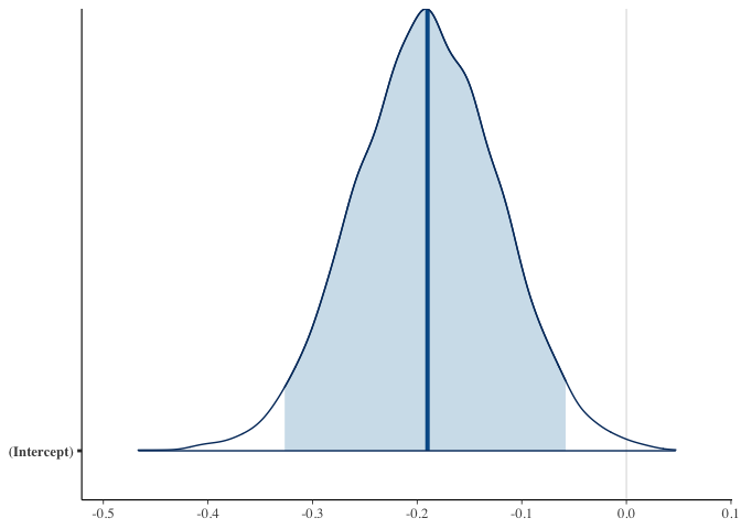
The Adjusted Log Odds coefficient is clearly positive. It is also almost certainly greater than 1, which means the slope is steeper that what you would expect if the Fight Odds perfectly tracked the Probability of the Favorite Winning. Indeed, this steep slope along with the negative intercept manifests in the clear trend whereby the Adjusted Odds overestimate mild Favorites but underestimate large ones.
plot(fit_5, plotfun = "areas", prob = 0.95,
     pars = "Adjust_Log_Odds")
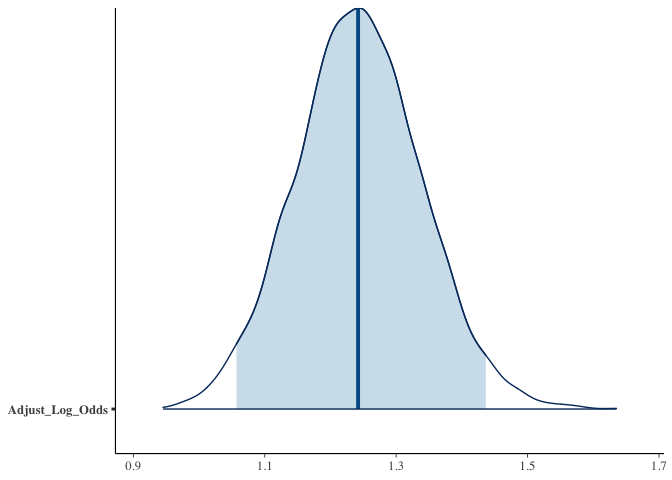
prob_reach_neg = round(mean(sims_5[, 3] < 0) * 100)
By analyzing the coefficient simulations, we can see that there is approximately a 2% probability that the effect of Reach is negative.
plot(fit_5, plotfun = "areas", prob = 0.95,
     pars = "Delta_REACH_imp")
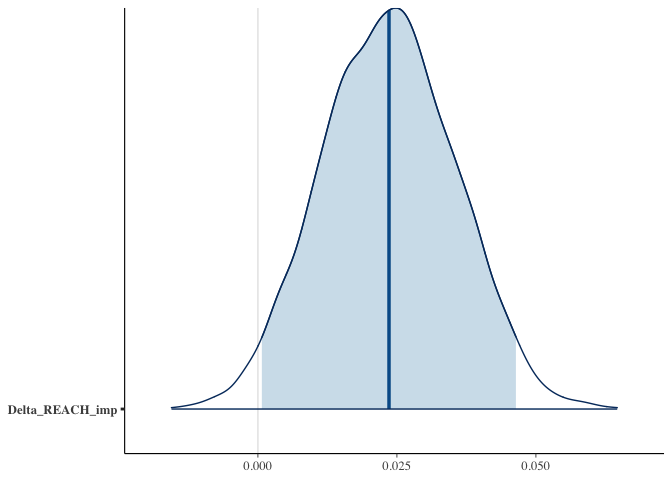
Save Best Model
Save best model - the one with two predictors: Adjusted Log Odds and (imputed) Difference in Fighter Reach.
save(fit_5, file = "./Models/bayesian_logistic_regression_two_predictor_model.RData")
Examine Predictions
Extract data frame from model object.
df <- fit_5$data
Extract fitted values.
df$predicted_prob <- fit_5$fitted.values
Predicted Outcomes
Compute predicted outcomes (i.e. if predicted probability of victory is greater than 50%).
df$predicted_fav_win <- ifelse(df$predicted_prob > 0.5, T, F)
Examine results table.
pred_table <- table(df$predicted_fav_win, df$Favorite_Won)
pred_table

##
##         FALSE TRUE
##   FALSE   182  182
##   TRUE    875 1749
Compute accuracy of the model.
right = (pred_table[1,1] + pred_table[2,2])  # underdog won and you predicted it plus the favorite won and you predicted it
wrong = (pred_table[2,1] + pred_table[1,2]) # underdog won and you did not predict it plus favorite won and you did not predict it

accuracy = right/(right + wrong)
accuracy

## [1] 0.6462517
Compute accuracy if you always pick favorite.
mean(df$Favorite_Won)

## [1] 0.6462517
Compute accuracy boost afforded by the model.
accuracy - mean(df$Favorite_Won)

## [1] 0
Predicted Bets
Compute predicted bets (note: this is different than predicted outcomes
-
with predicted bets we see if the predicted probability of victory exceeds the adjusted implied probability of victory of the odds).
df$predicted_bet_fav <- ifelse(df$predicted_prob > df$Adjust_Implied_Prob, T, F)
Get results table for predicted bets.
pred_table_bet <- table(df$predicted_bet_fav, df$Favorite_Won)
pred_table_bet

##
##         FALSE TRUE
##   FALSE   763 1018
##   TRUE    294  913
Get accuracy for predicted bets. Note: it is greater than chance (50%).
right_bet = (pred_table_bet[1,1] + pred_table_bet[2,2])  # underdog won and you bet on it plus the favorite won and you bet on it
wrong_bet = (pred_table_bet[2,1] + pred_table_bet[1,2]) # underdog won and you did not bet on it plus favorite won and you did not  bet on it

accuracy_bet = right_bet/(right_bet + wrong_bet)
accuracy_bet

## [1] 0.5609103
In-sample returns on predicted bets
Compute Potential Profit by converting Adjusted Implied Probabilities into decimal odds, with a standard 3% overround penalty (as an estimate since the overall overround is usually around 5% total). Also, compute potential profit without penalty.
df$Potential_Profit <- ifelse(df$Favorite_Won, 1/(df$Adjust_Implied_Prob + 0.03) - 1, 1/(1-df$Adjust_Implied_Prob + 0.03) - 1)
Compute actual profit.
df$Profit <- ifelse(
  (df$predicted_bet_fav & df$Favorite_Won) | (!(df$predicted_bet_fav) & !(df$Favorite_Won))
  , df$Potential_Profit
  , -1
  )
Compute ROI (%) based on in-sample predicted bets.
mean(df$Profit)

## [1] -0.01736408
Compute actual profit for just picking Favorites, and for just picking Underdogs.
df$Profit_Fav <- ifelse(
  df$Favorite_Won
  , df$Potential_Profit
  , -1
)

df$Profit_Dog <- ifelse(
  !(df$Favorite_Won)
  , df$Potential_Profit
  , -1
)
Compute ROI (%) for Favorite-only betting strategy.
mean(df$Profit_Fav)

## [1] -0.06242702
Compute ROI (%) for Underdog-only betting strategy.
mean(df$Profit_Dog)

## [1] -0.08220306
Conclusion
From a betting standpoint, the model cannot even overcome a modest average overround. Moreover, that is just for in-sample estimates - performance would be even worst with cross-validation estimates. On the other hand, the model does appear to substantially outperform simple / blind algorithms (such as just picking Favorites or just picking Underdogs). Practically, overcoming most of the overround (assuming 6% total and assuming the out-sample benefits are similar) may still confer some benefits as part of a larger betting strategy.