Fight Odds Analysis

Description

This script analyzes UFC fight odds data.

Libraries

library(tidyverse)
library(knitr)

Examine Data

Load data.

load("./Datasets/df_master.RData")

Get summary.

summary(df_master)

##      NAME               Date              Event               City          
##  Length:5986        Length:5986        Length:5986        Length:5986       
##  Class :character   Class :character   Class :character   Class :character  
##  Mode  :character   Mode  :character   Mode  :character   Mode  :character  
##                                                                             
##                                                                             
##                                                                             
##                                                                             
##     State             Country          FightWeightClass       Round     
##  Length:5986        Length:5986        Length:5986        Min.   :1.00  
##  Class :character   Class :character   Class :character   1st Qu.:1.00  
##  Mode  :character   Mode  :character   Mode  :character   Median :3.00  
##                                                           Mean   :2.43  
##                                                           3rd Qu.:3.00  
##                                                           Max.   :5.00  
##                                                                         
##     Method          Winner_Odds         Loser_Odds            Sex           
##  Length:5986        Length:5986        Length:5986        Length:5986       
##  Class :character   Class :character   Class :character   Class :character  
##  Mode  :character   Mode  :character   Mode  :character   Mode  :character  
##                                                                             
##                                                                             
##                                                                             
##                                                                             
##     fight_id       Result          FighterWeight   FighterWeightClass
##  Min.   :   1   Length:5986        Min.   :115.0   Length:5986       
##  1st Qu.: 749   Class :character   1st Qu.:135.0   Class :character  
##  Median :1497   Mode  :character   Median :155.0   Mode  :character  
##  Mean   :1497                      Mean   :163.8                     
##  3rd Qu.:2245                      3rd Qu.:185.0                     
##  Max.   :2993                      Max.   :265.0                     
##                                                                      
##      REACH            SLPM             SAPM             STRA       
##  Min.   :58.00   Min.   : 0.000   Min.   : 0.100   Min.   :0.0000  
##  1st Qu.:69.00   1st Qu.: 2.680   1st Qu.: 2.630   1st Qu.:0.3900  
##  Median :72.00   Median : 3.440   Median : 3.230   Median :0.4400  
##  Mean   :71.77   Mean   : 3.531   Mean   : 3.435   Mean   :0.4417  
##  3rd Qu.:75.00   3rd Qu.: 4.250   3rd Qu.: 4.030   3rd Qu.:0.4900  
##  Max.   :84.00   Max.   :11.140   Max.   :23.330   Max.   :0.8800  
##  NA's   :215                                                       
##       STRD              TD              TDA              TDD        
##  Min.   :0.0900   Min.   : 0.000   Min.   :0.0000   Min.   :0.0000  
##  1st Qu.:0.5100   1st Qu.: 0.560   1st Qu.:0.2700   1st Qu.:0.5100  
##  Median :0.5600   Median : 1.210   Median :0.3700   Median :0.6400  
##  Mean   :0.5527   Mean   : 1.518   Mean   :0.3745   Mean   :0.6157  
##  3rd Qu.:0.6000   3rd Qu.: 2.160   3rd Qu.:0.5000   3rd Qu.:0.7600  
##  Max.   :0.9200   Max.   :14.190   Max.   :1.0000   Max.   :1.0000  
##                                                                     
##       SUBA        
##  Min.   : 0.0000  
##  1st Qu.: 0.1000  
##  Median : 0.4000  
##  Mean   : 0.5516  
##  3rd Qu.: 0.8000  
##  Max.   :12.1000  
## 

Redefine variables.

df_master$NAME = as.factor(df_master$NAME)
df_master$Date = as.Date(df_master$Date)
df_master$Event = as.factor(df_master$Event)
df_master$City= as.factor(df_master$City)
df_master$State = as.factor(df_master$State)
df_master$Country = as.factor(df_master$Country)
df_master$FightWeightClass = as.factor(df_master$FightWeightClass)
df_master$Method = as.factor(df_master$Method)
df_master$Winner_Odds = as.numeric(df_master$Winner_Odds)
df_master$Loser_Odds = as.numeric(df_master$Loser_Odds)
df_master$fight_id = as.factor(df_master$fight_id)
df_master$Sex = as.factor(df_master$Sex)
df_master$Result = as.factor(df_master$Result)
df_master$FighterWeightClass = as.factor(df_master$FighterWeightClass)

Summarize again… There are infinite odds and overturned / DQ fight outcomes. These will have to be removed.

summary(df_master)

##                  NAME           Date           
##  Donald Cerrone    :  24   Min.   :2013-04-27  
##  Ovince Saint Preux:  21   1st Qu.:2015-08-23  
##  Jim Miller        :  19   Median :2017-05-28  
##  Neil Magny        :  19   Mean   :2017-06-19  
##  Derrick Lewis     :  18   3rd Qu.:2019-04-20  
##  Tim Means         :  18   Max.   :2021-02-06  
##  (Other)           :5867                       
##                                   Event                  City     
##  UFC Fight Night: Chiesa vs. Magny   :  28   Las Vegas     :1246  
##  UFC Fight Night: Poirier vs. Gaethje:  28   Abu Dhabi     : 258  
##  UFC Fight Night: Whittaker vs. Till :  28   Boston        : 124  
##  UFC 190: Rousey vs Correia          :  26   Rio de Janeiro: 124  
##  UFC 193: Rousey vs Holm             :  26   Chicago       : 118  
##  UFC 210: Cormier vs. Johnson 2      :  26   Newark        : 114  
##  (Other)                             :5824   (Other)       :4002  
##         State                      Country          FightWeightClass
##  Nevada    :1246   USA                 :3464   Welterweight : 986   
##  Abu Dhabi : 258   Brazil              : 532   Lightweight  : 984   
##  Texas     : 256   Canada              : 378   Bantamweight : 852   
##  New York  : 252   United Arab Emirates: 258   Featherweight: 724   
##  California: 250   Australia           : 236   Middleweight : 654   
##  Florida   : 176   United Kingdom      : 184   Flyweight    : 498   
##  (Other)   :3548   (Other)             : 934   (Other)      :1288   
##      Round             Method      Winner_Odds     Loser_Odds       Sex      
##  Min.   :1.00   DQ        :  14   Min.   :1.06   Min.   :1.07   Female: 766  
##  1st Qu.:1.00   KO/TKO    :1910   1st Qu.:1.42   1st Qu.:1.77   Male  :5220  
##  Median :3.00   M-DEC     :  34   Median :1.71   Median :2.38                
##  Mean   :2.43   Overturned:  20   Mean   : Inf   Mean   : Inf                
##  3rd Qu.:3.00   S-DEC     : 628   3rd Qu.:2.33   3rd Qu.:3.36                
##  Max.   :5.00   SUB       :1060   Max.   : Inf   Max.   : Inf                
##                 U-DEC     :2320                                              
##     fight_id       Result     FighterWeight       FighterWeightClass
##  1      :   2   Loser :2993   Min.   :115.0   Welterweight :1007    
##  2      :   2   Winner:2993   1st Qu.:135.0   Lightweight  : 980    
##  3      :   2                 Median :155.0   Bantamweight : 799    
##  4      :   2                 Mean   :163.8   Featherweight: 731    
##  5      :   2                 3rd Qu.:185.0   Middleweight : 659    
##  6      :   2                 Max.   :265.0   Flyweight    : 561    
##  (Other):5974                                 (Other)      :1249    
##      REACH            SLPM             SAPM             STRA       
##  Min.   :58.00   Min.   : 0.000   Min.   : 0.100   Min.   :0.0000  
##  1st Qu.:69.00   1st Qu.: 2.680   1st Qu.: 2.630   1st Qu.:0.3900  
##  Median :72.00   Median : 3.440   Median : 3.230   Median :0.4400  
##  Mean   :71.77   Mean   : 3.531   Mean   : 3.435   Mean   :0.4417  
##  3rd Qu.:75.00   3rd Qu.: 4.250   3rd Qu.: 4.030   3rd Qu.:0.4900  
##  Max.   :84.00   Max.   :11.140   Max.   :23.330   Max.   :0.8800  
##  NA's   :215                                                       
##       STRD              TD              TDA              TDD        
##  Min.   :0.0900   Min.   : 0.000   Min.   :0.0000   Min.   :0.0000  
##  1st Qu.:0.5100   1st Qu.: 0.560   1st Qu.:0.2700   1st Qu.:0.5100  
##  Median :0.5600   Median : 1.210   Median :0.3700   Median :0.6400  
##  Mean   :0.5527   Mean   : 1.518   Mean   :0.3745   Mean   :0.6157  
##  3rd Qu.:0.6000   3rd Qu.: 2.160   3rd Qu.:0.5000   3rd Qu.:0.7600  
##  Max.   :0.9200   Max.   :14.190   Max.   :1.0000   Max.   :1.0000  
##                                                                     
##       SUBA        
##  Min.   : 0.0000  
##  1st Qu.: 0.1000  
##  Median : 0.4000  
##  Mean   : 0.5516  
##  3rd Qu.: 0.8000  
##  Max.   :12.1000  
## 

How many events does the dataset include?

length(unique(df_master$Event))

## [1] 261

How many fights?

length(unique(df_master$fight_id))

## [1] 2993

Over what time frame?

range(sort(unique(df_master$Date)))

## [1] "2013-04-27" "2021-02-06"

Analyse Odds

Make copy for analysis.

df_odds = df_master
rm(df_master)

Filter out controversial results and infinite odds.

df_odds %>%
  dplyr::filter(
    (Method != "DQ") & (Method != "Overturned")
    , is.finite(Winner_Odds)
    , is.finite(Loser_Odds)
  ) -> df_odds

Get rid of fighter-specifics so that we can spread the data frame. This will give us one event per row.

df_odds %>%
  dplyr::select(-c(FighterWeight:SUBA)) %>%
  spread(Result, NAME) -> df_odds_short

How often were the (best) odds equal?

mean(df_odds$Winner_Odds == df_odds$Loser_Odds)

## [1] 0.005410889

sum(df_odds$Winner_Odds == df_odds$Loser_Odds)

## [1] 32

Filter out equal odds and identify if Favorite won the fight.

df_odds_short %>%
  dplyr::filter(Winner_Odds != Loser_Odds) %>%  # filter out equal odds
  dplyr::mutate(
    Favorite_was_Winner = ifelse(Winner_Odds < Loser_Odds, T, F)
    , Favorite_Unit_Profit = ifelse(Favorite_was_Winner, Winner_Odds - 1, -1)
    , Underdog_Unit_Profit = ifelse(!Favorite_was_Winner, Winner_Odds - 1, -1)
  ) -> df_odds_short

What was the mean unit profit (i.e. ROI) if one bet solely on the Favorite?

mean(df_odds_short$Favorite_Unit_Profit)

## [1] -0.02309419

What was the mean unit profit if one bet solely on the Underdog?

mean(df_odds_short$Underdog_Unit_Profit)

## [1] -0.002040122

What proportion of the time does the Favorite win?

mean(df_odds_short$Favorite_was_Winner)

## [1] 0.6460388

Calculate implied probability of each fight based on odds.

df_odds_short %>% dplyr::mutate(
  Favorite_Probability = ifelse(Favorite_was_Winner, 1/Winner_Odds, 1/Loser_Odds)
  , Underdog_Probability = ifelse(!Favorite_was_Winner,  1/Winner_Odds, 1/Loser_Odds)
) -> df_odds_short

Calculate overround for each fight.

NOTE: these odds are the best available odds for each fight / fighter. Therefore, this is not overround in the traditional sense (looking at one particular odds maker).

df_odds_short %>%
  dplyr::mutate(
    Total_Probability = Favorite_Probability + Underdog_Probability
    , Overround = Total_Probability - 1
  ) -> df_odds_short

There is very little overround. This is because we are picking the best odds for each fight / fighter. By picking the best odds, we are counteracting the built-in overround of any particular odds-maker (typically around 5% as a rough estimate).

mean(df_odds_short$Overround)

## [1] 0.004461755

mean(df_odds_short$Total_Probability)

## [1] 1.004462

Odds Performance

Add year as variable.

df_odds_short %>%
  dplyr::mutate(
    Year = format(Date,"%Y")
  ) -> df_odds_short

Compute Adjusted Implied Probability to account for the overround and get an unbiased estimate of the probability of victory implied by the odds.

df_odds_short %>%
  dplyr::mutate(
    Adjusted_Favorite_Probability = Favorite_Probability - Overround/2
    , Adjusted_Underdog_Probability = Underdog_Probability - Overround/2
    , Adjusted_Total_Probability = Adjusted_Favorite_Probability + Adjusted_Underdog_Probability
  ) -> df_odds_short

Looking at summary, we see that Adjusted Total Probability is always equal to 100%. Moreover, the Favorite Probability never dips below 50%, whereas the Underdog Probability never exceeds it.

summary(df_odds_short)

##       Date                                             Event     
##  Min.   :2013-04-27   UFC Fight Night: Chiesa vs. Magny   :  14  
##  1st Qu.:2015-08-23   UFC Fight Night: Poirier vs. Gaethje:  14  
##  Median :2017-05-13   UFC Fight Night: Whittaker vs. Till :  14  
##  Mean   :2017-06-17   UFC 190: Rousey vs Correia          :  13  
##  3rd Qu.:2019-04-20   UFC 193: Rousey vs Holm             :  13  
##  Max.   :2021-02-06   UFC 210: Cormier vs. Johnson 2      :  13  
##                       (Other)                             :2860  
##              City             State                      Country    
##  Las Vegas     : 607   Nevada    : 607   USA                 :1699  
##  Abu Dhabi     : 127   Abu Dhabi : 127   Brazil              : 258  
##  Rio de Janeiro:  60   Texas     : 127   Canada              : 187  
##  Boston        :  59   California: 123   United Arab Emirates: 127  
##  Chicago       :  57   New York  : 123   Australia           : 117  
##  Newark        :  57   Florida   :  88   United Kingdom      :  92  
##  (Other)       :1974   (Other)   :1746   (Other)             : 461  
##       FightWeightClass     Round              Method      Winner_Odds    
##  Welterweight :486     Min.   :1.000   DQ        :   0   Min.   : 1.060  
##  Lightweight  :484     1st Qu.:2.000   KO/TKO    : 942   1st Qu.: 1.420  
##  Bantamweight :420     Median :3.000   M-DEC     :  17   Median : 1.710  
##  Featherweight:355     Mean   :2.435   Overturned:   0   Mean   : 1.975  
##  Middleweight :316     3rd Qu.:3.000   S-DEC     : 312   3rd Qu.: 2.300  
##  Flyweight    :246     Max.   :5.000   SUB       : 521   Max.   :12.990  
##  (Other)      :634                     U-DEC     :1149                   
##    Loser_Odds         Sex          fight_id                Loser     
##  Min.   : 1.070   Female: 378   1      :   1   Jim Miller     :  10  
##  1st Qu.: 1.760   Male  :2563   2      :   1   Ross Pearson   :  10  
##  Median : 2.380                 3      :   1   Angela Hill    :   9  
##  Mean   : 2.813                 4      :   1   Donald Cerrone :   9  
##  3rd Qu.: 3.350                 5      :   1   Gian Villante  :   9  
##  Max.   :14.050                 6      :   1   Jeremy Stephens:   9  
##                                 (Other):2935   (Other)        :2885  
##                 Winner     Favorite_was_Winner Favorite_Unit_Profit
##  Donald Cerrone    :  15   Mode :logical       Min.   :-1.00000    
##  Derrick Lewis     :  14   FALSE:1041          1st Qu.:-1.00000    
##  Francisco Trinaldo:  13   TRUE :1900          Median : 0.31000    
##  Neil Magny        :  13                       Mean   :-0.02309    
##  Dustin Poirier    :  12                       3rd Qu.: 0.57000    
##  Max Holloway      :  12                       Max.   : 1.10000    
##  (Other)           :2862                                           
##  Underdog_Unit_Profit Favorite_Probability Underdog_Probability
##  Min.   :-1.00000     Min.   :0.4000       Min.   :0.07117     
##  1st Qu.:-1.00000     1st Qu.:0.5780       1st Qu.:0.27397     
##  Median :-1.00000     Median :0.6410       Median :0.35971     
##  Mean   :-0.00204     Mean   :0.6579       Mean   :0.34658     
##  3rd Qu.: 1.30000     3rd Qu.:0.7299       3rd Qu.:0.42553     
##  Max.   :11.99000     Max.   :0.9434       Max.   :0.52356     
##                                                                
##  Total_Probability   Overround             Year          
##  Min.   :0.7639    Min.   :-0.236148   Length:2941       
##  1st Qu.:0.9988    1st Qu.:-0.001198   Class :character  
##  Median :1.0085    Median : 0.008472   Mode  :character  
##  Mean   :1.0045    Mean   : 0.004462                     
##  3rd Qu.:1.0147    3rd Qu.: 0.014713                     
##  Max.   :1.0684    Max.   : 0.068376                     
##                                                          
##  Adjusted_Favorite_Probability Adjusted_Underdog_Probability
##  Min.   :0.5012                Min.   :0.0673               
##  1st Qu.:0.5780                1st Qu.:0.2725               
##  Median :0.6408                Median :0.3592               
##  Mean   :0.6557                Mean   :0.3443               
##  3rd Qu.:0.7275                3rd Qu.:0.4220               
##  Max.   :0.9327                Max.   :0.4988               
##                                                             
##  Adjusted_Total_Probability
##  Min.   :1                 
##  1st Qu.:1                 
##  Median :1                 
##  Mean   :1                 
##  3rd Qu.:1                 
##  Max.   :1                 
## 

Create function to graphically assess over performance as a function of several variables. These are not inferential analyses but are instead meant to visualize the data to observe trends for further analysis. Use adjusted implied probabilities along with unit profits derived from non-adjusted odds to simulate what one actually would have won using best available odds.

gauge_over_performance = function(num_bin = 10, min_bin_size = 30, variable = NULL) {

  # get bins for Favorite
  df_odds_short$Favorite_Probability_Bin = cut(df_odds_short$Adjusted_Favorite_Probability, num_bin)
  # get bins for Underdog
  df_odds_short$Underdog_Probability_Bin = cut(df_odds_short$Adjusted_Underdog_Probability, num_bin)

  if (is.null(variable)) {
    # check over/under performance for Favorites
    df_odds_short %>%
      dplyr::group_by(Favorite_Probability_Bin) %>%
      dplyr::summarise(
        Prop_of_Victory = mean(Favorite_was_Winner)
        , Size_of_Bin = length(Favorite_was_Winner)
        , ROI = mean(Favorite_Unit_Profit)
      ) -> fav_perf
  } else {

    # create dummy variable for function
    df_odds_short$Dummy = df_odds_short[
      ,which(colnames(df_odds_short) == sprintf("%s", variable))
    ]

    # check over/under performance for Favorites
    df_odds_short %>%
      dplyr::group_by(Favorite_Probability_Bin, Dummy) %>%
      dplyr::summarise(
        Prop_of_Victory = mean(Favorite_was_Winner)
        , Size_of_Bin = length(Favorite_was_Winner)
        , ROI = mean(Favorite_Unit_Profit)
      ) -> fav_perf
  }

  # extract bins
  fav_labs <- as.character(fav_perf$Favorite_Probability_Bin)
  fav_bins = as.data.frame(
    cbind(
      lower = as.numeric( sub("\\((.+),.*", "\\1", fav_labs) )
      , upper = as.numeric( sub("[^,]*,([^]]*)\\]", "\\1", fav_labs) )
    )
  )
  # get value in middle of bin
  fav_bins %>% dplyr::mutate(mid_bin = (lower + upper)/2 ) -> fav_bins
  # add mid bin column
  fav_perf$Mid_Bin = fav_bins$mid_bin
  # add Over performance column
  fav_perf %>% dplyr::mutate(Over_Performance = Prop_of_Victory - Mid_Bin) -> fav_perf


  if (is.null(variable)) {

    # plot over/under performance
    fav_perf %>%
      dplyr::filter(Size_of_Bin >= min_bin_size) %>%
      ggplot(aes(x=Mid_Bin*100, y=Over_Performance * 100))+
      geom_point()+
      geom_smooth(se=F)+
      geom_hline(yintercept = 0, linetype = "dotted")+
      ylab("Over Performance (%)")+
      xlab("Adjusted Implied Probability (%)")+
      ggtitle("Favorites")->gg
    print(gg)

    # plot over/under performance
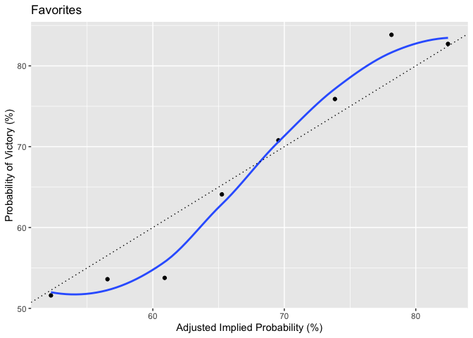
    fav_perf %>%
      dplyr::filter(Size_of_Bin >= min_bin_size) %>%
      ggplot(aes(x=Mid_Bin * 100, y=Prop_of_Victory*100))+
      geom_point()+
      geom_smooth(se=F)+
      ylab("Probability of Victory (%)")+
      xlab("Adjusted Implied Probability (%)")+
      geom_abline(slope=1, intercept=0, linetype = "dotted")+
      ggtitle("Favorites")->gg
    print(gg)

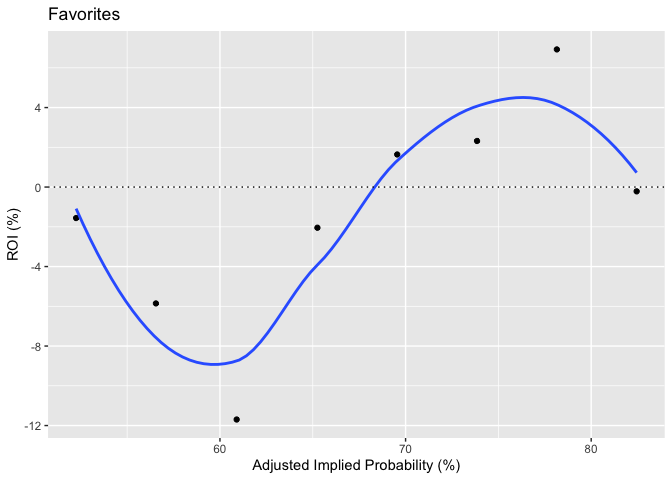
    # plot ROI - only real difference is scale along y axis
    fav_perf %>%
      dplyr::filter(Size_of_Bin >= min_bin_size) %>%
      ggplot(aes(x=Mid_Bin*100, y= ROI* 100))+
      geom_point()+
      geom_smooth(se=F)+
      geom_hline(yintercept = 0, linetype = "dotted")+
      ylab("ROI (%)")+
      xlab("Adjusted Implied Probability (%)")+
      ggtitle("Favorites") -> gg
    print(gg)

  } else {
    # plot over/under performance
    fav_perf %>%
      dplyr::filter(Size_of_Bin >= min_bin_size) %>%
      ggplot(aes(x=Mid_Bin*100, y=Over_Performance * 100, group=Dummy, colour = Dummy))+
      geom_point()+
      geom_smooth(se=F)+
      geom_hline(yintercept = 0, linetype = "dotted")+
      ylab("Over Performance (%)")+
      xlab("Adjusted Implied Probability (%)")+
      ggtitle("Favorites")+
      labs(color=sprintf("%s", variable)) -> gg
    print(gg)

    # plot ROI - only real difference is scale along y axis
    fav_perf %>%
      dplyr::filter(Size_of_Bin >= min_bin_size) %>%
      ggplot(aes(x=Mid_Bin*100, y= ROI* 100, group=Dummy, colour = Dummy))+
      geom_point()+
      geom_smooth(se=F)+
      geom_hline(yintercept = 0, linetype = "dotted")+
      ylab("ROI (%)")+
      xlab("Adjusted Implied Probability (%)")+
      ggtitle("Favorites")+
      labs(color=sprintf("%s", variable)) -> gg
    print(gg)
  }


  if (is.null(variable)) {

    # check over/under performance for Underdogs
    df_odds_short %>%
      dplyr::group_by(Underdog_Probability_Bin) %>%
      dplyr::summarise(
        Prop_of_Victory = mean(!Favorite_was_Winner)
        , Size_of_Bin = length(!Favorite_was_Winner)
        , ROI = mean(Underdog_Unit_Profit)
      ) -> under_perf

  } else {

    # check over/under performance for Underdogs
    df_odds_short %>%
      dplyr::group_by(Underdog_Probability_Bin, Dummy) %>%
      dplyr::summarise(
        Prop_of_Victory = mean(!Favorite_was_Winner)
        , Size_of_Bin = length(!Favorite_was_Winner)
        , ROI = mean(Underdog_Unit_Profit)
      ) -> under_perf
  }

  # extract bins
  under_labs <- as.character(under_perf$Underdog_Probability_Bin)
  under_bins = as.data.frame(
    cbind(
      lower = as.numeric( sub("\\((.+),.*", "\\1", under_labs) )
      , upper = as.numeric( sub("[^,]*,([^]]*)\\]", "\\1", under_labs) )
    )
  )
  # get value in middle of bin
  under_bins %>% dplyr::mutate(mid_bin = (lower + upper)/2 ) -> under_bins
  # add mid bin column
  under_perf$Mid_Bin = under_bins$mid_bin
  # add Over performance column
  under_perf %>% dplyr::mutate(Over_Performance = Prop_of_Victory - Mid_Bin) -> under_perf


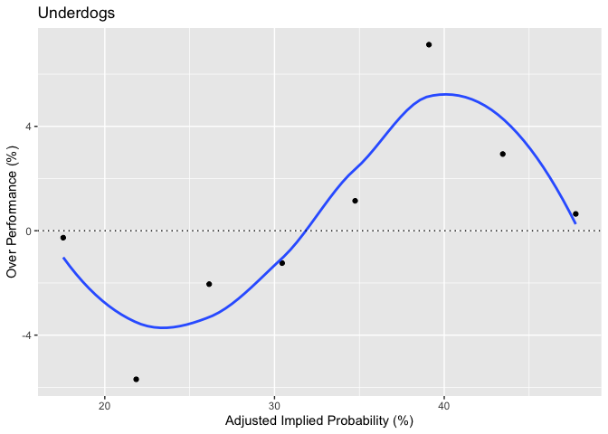
  if (is.null(variable)) {
    # plot over/under performance
    under_perf %>%
      dplyr::filter(Size_of_Bin >= min_bin_size) %>%
      ggplot(aes(x=Mid_Bin*100, y=Over_Performance * 100))+
      geom_point()+
      geom_smooth(se=F)+
      geom_hline(yintercept = 0, linetype = "dotted")+
      ylab("Over Performance (%)")+
      xlab("Adjusted Implied Probability (%)")+
      ggtitle("Underdogs")->gg
    print(gg)

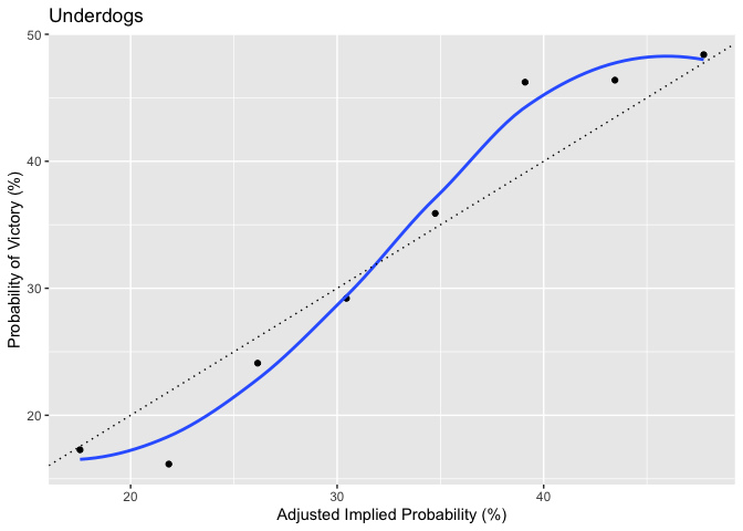
    # plot over/under performance
    under_perf %>%
      dplyr::filter(Size_of_Bin >= min_bin_size) %>%
      ggplot(aes(x=Mid_Bin * 100, y=Prop_of_Victory*100))+
      geom_point()+
      geom_smooth(se=F)+
      ylab("Probability of Victory (%)")+
      xlab("Adjusted Implied Probability (%)")+
      geom_abline(slope=1, intercept=0, linetype = "dotted")+
      ggtitle("Underdogs")->gg
    print(gg)

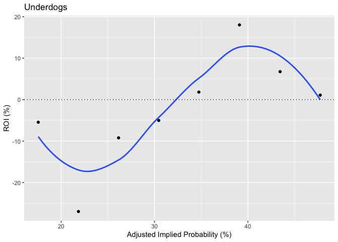
    under_perf %>%
      dplyr::filter(Size_of_Bin >= min_bin_size) %>%
      ggplot(aes(x=Mid_Bin*100, y=ROI * 100))+
      geom_point()+
      geom_smooth(se=F)+
      geom_hline(yintercept = 0, linetype = "dotted")+
      ylab("ROI (%)")+
      xlab("Adjusted Implied Probability (%)")+
      ggtitle("Underdogs")-> gg
    print(gg)

  } else {

    # plot over/under performance
    under_perf %>%
      dplyr::filter(Size_of_Bin >= min_bin_size) %>%
      ggplot(aes(x=Mid_Bin*100, y=Over_Performance * 100, group=Dummy, colour = Dummy))+
      geom_point()+
      geom_smooth(se=F)+
      geom_hline(yintercept = 0, linetype = "dotted")+
      ylab("Over Performance (%)")+
      xlab("Adjusted Implied Probability (%)")+
      ggtitle("Underdogs")+
      labs(color=sprintf("%s", variable)) -> gg
    print(gg)

    under_perf %>%
      dplyr::filter(Size_of_Bin >= min_bin_size) %>%
      ggplot(aes(x=Mid_Bin*100, y=ROI * 100, group=Dummy, colour = Dummy))+
      geom_point()+
      geom_smooth(se=F)+
      geom_hline(yintercept = 0, linetype = "dotted")+
      ylab("ROI (%)")+
      xlab("Adjusted Implied Probability (%)")+
      ggtitle("Underdogs")+
      labs(color=sprintf("%s", variable)) -> gg
    print(gg)
  }
  
  # process to return()
  under_perf$Is_Fav = F
  under_perf %>%
    rename(Probability_Bin = Underdog_Probability_Bin) -> under_perf
  
  fav_perf$Is_Fav = T
  fav_perf %>%
    rename(Probability_Bin = Favorite_Probability_Bin) -> fav_perf
  
  return(rbind(fav_perf, under_perf))

}

Look at how expected performance predicts over performance.

odds_perf = gauge_over_performance(num_bin = 10, min_bin_size = 100, variable = NULL)

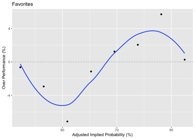
kable(odds_perf)

Probability_Bin	Prop_of_Victory	Size_of_Bin	ROI	Mid_Bin	Over_Performance	Is_Fav
(0.501,0.544]	0.5160494	405	-0.0155802	0.52250	-0.0064506	TRUE
(0.544,0.587]	0.5361050	457	-0.0585558	0.56550	-0.0293950	TRUE
(0.587,0.631]	0.5376984	504	-0.1169643	0.60900	-0.0713016	TRUE
(0.631,0.674]	0.6410256	390	-0.0204615	0.65250	-0.0114744	TRUE
(0.674,0.717]	0.7078947	380	0.0163947	0.69550	0.0123947	TRUE
(0.717,0.76]	0.7589577	307	0.0231922	0.73850	0.0204577	TRUE
(0.76,0.803]	0.8384279	229	0.0692576	0.78150	0.0569279	TRUE
(0.803,0.846]	0.8271605	162	-0.0021605	0.82450	0.0026605	TRUE
(0.846,0.89]	0.8961039	77	0.0325974	0.86800	0.0281039	TRUE
(0.89,0.933]	0.9333333	30	0.0236667	0.91150	0.0218333	TRUE
(0.0669,0.11]	0.0666667	30	-0.2100000	0.08845	-0.0217833	FALSE
(0.11,0.154]	0.1038961	77	-0.1935065	0.13200	-0.0281039	FALSE
(0.154,0.197]	0.1728395	162	-0.0545062	0.17550	-0.0026605	FALSE
(0.197,0.24]	0.1615721	229	-0.2699127	0.21850	-0.0569279	FALSE
(0.24,0.283]	0.2410423	307	-0.0922150	0.26150	-0.0204577	FALSE
(0.283,0.326]	0.2921053	380	-0.0502105	0.30450	-0.0123947	FALSE
(0.326,0.369]	0.3589744	390	0.0181795	0.34750	0.0114744	FALSE
(0.369,0.413]	0.4623016	504	0.1802976	0.39100	0.0713016	FALSE
(0.413,0.456]	0.4638950	457	0.0675055	0.43450	0.0293950	FALSE
(0.456,0.499]	0.4839506	405	0.0109136	0.47750	0.0064506	FALSE

Is there any stability across years? Need to reduce minimum bin size to get estimates. As a result, estimates will be more noisy.

odds_perf_by_year = gauge_over_performance(num_bin = 10, min_bin_size = 30, variable = "Year")

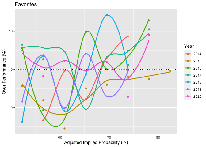
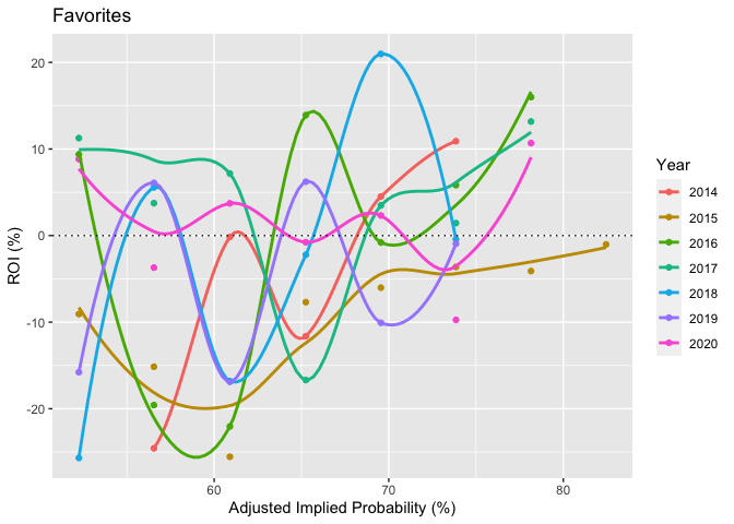
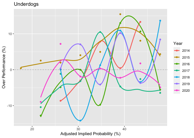
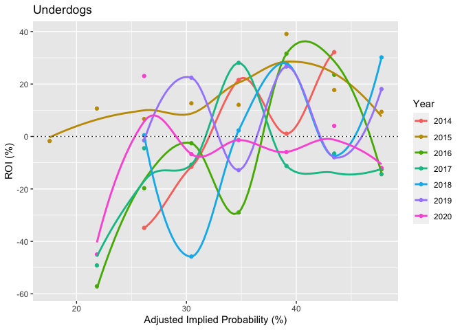
kable(odds_perf_by_year)

Probability_Bin	Dummy	Prop_of_Victory	Size_of_Bin	ROI	Mid_Bin	Over_Performance	Is_Fav
(0.501,0.544]	2013	0.6000000	10	0.1580000	0.52250	0.0775000	TRUE
(0.501,0.544]	2014	0.6086957	23	0.1791304	0.52250	0.0861957	TRUE
(0.501,0.544]	2015	0.4791667	48	-0.0906250	0.52250	-0.0433333	TRUE
(0.501,0.544]	2016	0.5777778	90	0.0936667	0.52250	0.0552778	TRUE
(0.501,0.544]	2017	0.5869565	46	0.1126087	0.52250	0.0644565	TRUE
(0.501,0.544]	2018	0.3859649	57	-0.2568421	0.52250	-0.1365351	TRUE
(0.501,0.544]	2019	0.4383562	73	-0.1578082	0.52250	-0.0841438	TRUE
(0.501,0.544]	2020	0.5714286	56	0.0882143	0.52250	0.0489286	TRUE
(0.501,0.544]	2021	0.5000000	2	-0.0250000	0.52250	-0.0225000	TRUE
(0.544,0.587]	2013	0.4444444	9	-0.1977778	0.56550	-0.1210556	TRUE
(0.544,0.587]	2014	0.4324324	37	-0.2456757	0.56550	-0.1330676	TRUE
(0.544,0.587]	2015	0.4848485	66	-0.1515152	0.56550	-0.0806515	TRUE
(0.544,0.587]	2016	0.4590164	61	-0.1957377	0.56550	-0.1064836	TRUE
(0.544,0.587]	2017	0.5915493	71	0.0374648	0.56550	0.0260493	TRUE
(0.544,0.587]	2018	0.6000000	55	0.0556364	0.56550	0.0345000	TRUE
(0.544,0.587]	2019	0.6025641	78	0.0608974	0.56550	0.0370641	TRUE
(0.544,0.587]	2020	0.5479452	73	-0.0369863	0.56550	-0.0175548	TRUE
(0.544,0.587]	2021	0.4285714	7	-0.2457143	0.56550	-0.1369286	TRUE
(0.587,0.631]	2013	0.5000000	18	-0.1722222	0.60900	-0.1090000	TRUE
(0.587,0.631]	2014	0.6046512	43	-0.0016279	0.60900	-0.0043488	TRUE
(0.587,0.631]	2015	0.4545455	66	-0.2554545	0.60900	-0.1544545	TRUE
(0.587,0.631]	2016	0.4791667	96	-0.2204167	0.60900	-0.1298333	TRUE
(0.587,0.631]	2017	0.6557377	61	0.0716393	0.60900	0.0467377	TRUE
(0.587,0.631]	2018	0.5000000	84	-0.1680952	0.60900	-0.1090000	TRUE
(0.587,0.631]	2019	0.5068493	73	-0.1689041	0.60900	-0.1021507	TRUE
(0.587,0.631]	2020	0.6315789	57	0.0371930	0.60900	0.0225789	TRUE
(0.587,0.631]	2021	0.8333333	6	0.3666667	0.60900	0.2243333	TRUE
(0.631,0.674]	2013	0.6666667	15	0.0280000	0.65250	0.0141667	TRUE
(0.631,0.674]	2014	0.5744681	47	-0.1161702	0.65250	-0.0780319	TRUE
(0.631,0.674]	2015	0.6029412	68	-0.0769118	0.65250	-0.0495588	TRUE
(0.631,0.674]	2016	0.7500000	56	0.1391071	0.65250	0.0975000	TRUE
(0.631,0.674]	2017	0.5476190	42	-0.1669048	0.65250	-0.1048810	TRUE
(0.631,0.674]	2018	0.6400000	50	-0.0222000	0.65250	-0.0125000	TRUE
(0.631,0.674]	2019	0.6938776	49	0.0622449	0.65250	0.0413776	TRUE
(0.631,0.674]	2020	0.6491228	57	-0.0077193	0.65250	-0.0033772	TRUE
(0.631,0.674]	2021	0.6666667	6	0.0016667	0.65250	0.0141667	TRUE
(0.674,0.717]	2013	0.8235294	17	0.2058824	0.69550	0.1280294	TRUE
(0.674,0.717]	2014	0.7254902	51	0.0450980	0.69550	0.0299902	TRUE
(0.674,0.717]	2015	0.6551724	58	-0.0601724	0.69550	-0.0403276	TRUE
(0.674,0.717]	2016	0.6956522	69	-0.0079710	0.69550	0.0001522	TRUE
(0.674,0.717]	2017	0.7272727	33	0.0348485	0.69550	0.0317727	TRUE
(0.674,0.717]	2018	0.8372093	43	0.2097674	0.69550	0.1417093	TRUE
(0.674,0.717]	2019	0.6250000	40	-0.1007500	0.69550	-0.0705000	TRUE
(0.674,0.717]	2020	0.7142857	63	0.0231746	0.69550	0.0187857	TRUE
(0.674,0.717]	2021	0.3333333	6	-0.5216667	0.69550	-0.3621667	TRUE
(0.717,0.76]	2013	0.9411765	17	0.2811765	0.73850	0.2026765	TRUE
(0.717,0.76]	2014	0.8250000	40	0.1090000	0.73850	0.0865000	TRUE
(0.717,0.76]	2015	0.7187500	32	-0.0362500	0.73850	-0.0197500	TRUE
(0.717,0.76]	2016	0.7872340	47	0.0582979	0.73850	0.0487340	TRUE
(0.717,0.76]	2017	0.7500000	48	0.0143750	0.73850	0.0115000	TRUE
(0.717,0.76]	2018	0.7380952	42	-0.0042857	0.73850	-0.0004048	TRUE
(0.717,0.76]	2019	0.7352941	34	-0.0094118	0.73850	-0.0032059	TRUE
(0.717,0.76]	2020	0.6666667	42	-0.0973810	0.73850	-0.0718333	TRUE
(0.717,0.76]	2021	0.8000000	5	0.0600000	0.73850	0.0615000	TRUE
(0.76,0.803]	2013	0.9090909	11	0.1609091	0.78150	0.1275909	TRUE
(0.76,0.803]	2014	0.7500000	24	-0.0437500	0.78150	-0.0315000	TRUE
(0.76,0.803]	2015	0.7560976	41	-0.0409756	0.78150	-0.0254024	TRUE
(0.76,0.803]	2016	0.9090909	33	0.1600000	0.78150	0.1275909	TRUE
(0.76,0.803]	2017	0.8857143	35	0.1317143	0.78150	0.1042143	TRUE
(0.76,0.803]	2018	0.8214286	28	0.0521429	0.78150	0.0399286	TRUE
(0.76,0.803]	2019	0.8400000	25	0.0748000	0.78150	0.0585000	TRUE
(0.76,0.803]	2020	0.8709677	31	0.1067742	0.78150	0.0894677	TRUE
(0.76,0.803]	2021	1.0000000	1	0.2900000	0.78150	0.2185000	TRUE
(0.803,0.846]	2013	0.8000000	10	-0.0350000	0.82450	-0.0245000	TRUE
(0.803,0.846]	2014	0.8571429	21	0.0380952	0.82450	0.0326429	TRUE
(0.803,0.846]	2015	0.8205128	39	-0.0102564	0.82450	-0.0039872	TRUE
(0.803,0.846]	2016	0.7368421	19	-0.1110526	0.82450	-0.0876579	TRUE
(0.803,0.846]	2017	0.7619048	21	-0.0819048	0.82450	-0.0625952	TRUE
(0.803,0.846]	2018	0.8636364	22	0.0309091	0.82450	0.0391364	TRUE
(0.803,0.846]	2019	0.8666667	15	0.0506667	0.82450	0.0421667	TRUE
(0.803,0.846]	2020	0.9166667	12	0.1108333	0.82450	0.0921667	TRUE
(0.803,0.846]	2021	1.0000000	3	0.2200000	0.82450	0.1755000	TRUE
(0.846,0.89]	2013	1.0000000	6	0.1500000	0.86800	0.1320000	TRUE
(0.846,0.89]	2014	0.8000000	15	-0.0713333	0.86800	-0.0680000	TRUE
(0.846,0.89]	2015	0.8823529	17	0.0088235	0.86800	0.0143529	TRUE
(0.846,0.89]	2016	1.0000000	5	0.1420000	0.86800	0.1320000	TRUE
(0.846,0.89]	2017	0.8571429	7	-0.0142857	0.86800	-0.0108571	TRUE
(0.846,0.89]	2018	1.0000000	10	0.1530000	0.86800	0.1320000	TRUE
(0.846,0.89]	2019	0.8750000	8	0.0150000	0.86800	0.0070000	TRUE
(0.846,0.89]	2020	0.8888889	9	0.0300000	0.86800	0.0208889	TRUE
(0.89,0.933]	2014	1.0000000	4	0.0900000	0.91150	0.0885000	TRUE
(0.89,0.933]	2015	0.8750000	8	-0.0487500	0.91150	-0.0365000	TRUE
(0.89,0.933]	2016	1.0000000	3	0.0933333	0.91150	0.0885000	TRUE
(0.89,0.933]	2017	1.0000000	3	0.1100000	0.91150	0.0885000	TRUE
(0.89,0.933]	2018	1.0000000	5	0.1080000	0.91150	0.0885000	TRUE
(0.89,0.933]	2019	1.0000000	4	0.1050000	0.91150	0.0885000	TRUE
(0.89,0.933]	2020	0.6666667	3	-0.2766667	0.91150	-0.2448333	TRUE
(0.0669,0.11]	2014	0.0000000	4	-1.0000000	0.08845	-0.0884500	FALSE
(0.0669,0.11]	2015	0.1250000	8	0.6237500	0.08845	0.0365500	FALSE
(0.0669,0.11]	2016	0.0000000	3	-1.0000000	0.08845	-0.0884500	FALSE
(0.0669,0.11]	2017	0.0000000	3	-1.0000000	0.08845	-0.0884500	FALSE
(0.0669,0.11]	2018	0.0000000	5	-1.0000000	0.08845	-0.0884500	FALSE
(0.0669,0.11]	2019	0.0000000	4	-1.0000000	0.08845	-0.0884500	FALSE
(0.0669,0.11]	2020	0.3333333	3	2.5700000	0.08845	0.2448833	FALSE
(0.11,0.154]	2013	0.0000000	6	-1.0000000	0.13200	-0.1320000	FALSE
(0.11,0.154]	2014	0.2000000	15	0.5980000	0.13200	0.0680000	FALSE
(0.11,0.154]	2015	0.1176471	17	-0.1276471	0.13200	-0.0143529	FALSE
(0.11,0.154]	2016	0.0000000	5	-1.0000000	0.13200	-0.1320000	FALSE
(0.11,0.154]	2017	0.1428571	7	-0.0671429	0.13200	0.0108571	FALSE
(0.11,0.154]	2018	0.0000000	10	-1.0000000	0.13200	-0.1320000	FALSE
(0.11,0.154]	2019	0.1250000	8	0.0937500	0.13200	-0.0070000	FALSE
(0.11,0.154]	2020	0.1111111	9	-0.1088889	0.13200	-0.0208889	FALSE
(0.154,0.197]	2013	0.2000000	10	0.0550000	0.17550	0.0245000	FALSE
(0.154,0.197]	2014	0.1428571	21	-0.2428571	0.17550	-0.0326429	FALSE
(0.154,0.197]	2015	0.1794872	39	-0.0174359	0.17550	0.0039872	FALSE
(0.154,0.197]	2016	0.2631579	19	0.4815789	0.17550	0.0876579	FALSE
(0.154,0.197]	2017	0.2380952	21	0.3666667	0.17550	0.0625952	FALSE
(0.154,0.197]	2018	0.1363636	22	-0.2586364	0.17550	-0.0391364	FALSE
(0.154,0.197]	2019	0.1333333	15	-0.3406667	0.17550	-0.0421667	FALSE
(0.154,0.197]	2020	0.0833333	12	-0.5541667	0.17550	-0.0921667	FALSE
(0.154,0.197]	2021	0.0000000	3	-1.0000000	0.17550	-0.1755000	FALSE
(0.197,0.24]	2013	0.0909091	11	-0.5772727	0.21850	-0.1275909	FALSE
(0.197,0.24]	2014	0.2500000	24	0.1258333	0.21850	0.0315000	FALSE
(0.197,0.24]	2015	0.2439024	41	0.1065854	0.21850	0.0254024	FALSE
(0.197,0.24]	2016	0.0909091	33	-0.5712121	0.21850	-0.1275909	FALSE
(0.197,0.24]	2017	0.1142857	35	-0.4914286	0.21850	-0.1042143	FALSE
(0.197,0.24]	2018	0.1785714	28	-0.1767857	0.21850	-0.0399286	FALSE
(0.197,0.24]	2019	0.1600000	25	-0.2760000	0.21850	-0.0585000	FALSE
(0.197,0.24]	2020	0.1290323	31	-0.4500000	0.21850	-0.0894677	FALSE
(0.197,0.24]	2021	0.0000000	1	-1.0000000	0.21850	-0.2185000	FALSE
(0.24,0.283]	2013	0.0588235	17	-0.7847059	0.26150	-0.2026765	FALSE
(0.24,0.283]	2014	0.1750000	40	-0.3487500	0.26150	-0.0865000	FALSE
(0.24,0.283]	2015	0.2812500	32	0.0665625	0.26150	0.0197500	FALSE
(0.24,0.283]	2016	0.2127660	47	-0.1972340	0.26150	-0.0487340	FALSE
(0.24,0.283]	2017	0.2500000	48	-0.0447917	0.26150	-0.0115000	FALSE
(0.24,0.283]	2018	0.2619048	42	0.0047619	0.26150	0.0004048	FALSE
(0.24,0.283]	2019	0.2647059	34	-0.0150000	0.26150	0.0032059	FALSE
(0.24,0.283]	2020	0.3333333	42	0.2304762	0.26150	0.0718333	FALSE
(0.24,0.283]	2021	0.2000000	5	-0.2200000	0.26150	-0.0615000	FALSE
(0.283,0.326]	2013	0.1764706	17	-0.4088235	0.30450	-0.1280294	FALSE
(0.283,0.326]	2014	0.2745098	51	-0.1156863	0.30450	-0.0299902	FALSE
(0.283,0.326]	2015	0.3448276	58	0.1263793	0.30450	0.0403276	FALSE
(0.283,0.326]	2016	0.3043478	69	-0.0256522	0.30450	-0.0001522	FALSE
(0.283,0.326]	2017	0.2727273	33	-0.1075758	0.30450	-0.0317727	FALSE
(0.283,0.326]	2018	0.1627907	43	-0.4579070	0.30450	-0.1417093	FALSE
(0.283,0.326]	2019	0.3750000	40	0.2240000	0.30450	0.0705000	FALSE
(0.283,0.326]	2020	0.2857143	63	-0.0673016	0.30450	-0.0187857	FALSE
(0.283,0.326]	2021	0.6666667	6	1.1216667	0.30450	0.3621667	FALSE
(0.326,0.369]	2013	0.3333333	15	-0.0546667	0.34750	-0.0141667	FALSE
(0.326,0.369]	2014	0.4255319	47	0.2155319	0.34750	0.0780319	FALSE
(0.326,0.369]	2015	0.3970588	68	0.1205882	0.34750	0.0495588	FALSE
(0.326,0.369]	2016	0.2500000	56	-0.2896429	0.34750	-0.0975000	FALSE
(0.326,0.369]	2017	0.4523810	42	0.2807143	0.34750	0.1048810	FALSE
(0.326,0.369]	2018	0.3600000	50	0.0230000	0.34750	0.0125000	FALSE
(0.326,0.369]	2019	0.3061224	49	-0.1281633	0.34750	-0.0413776	FALSE
(0.326,0.369]	2020	0.3508772	57	-0.0136842	0.34750	0.0033772	FALSE
(0.326,0.369]	2021	0.3333333	6	-0.0133333	0.34750	-0.0141667	FALSE
(0.369,0.413]	2013	0.5000000	18	0.2916667	0.39100	0.1090000	FALSE
(0.369,0.413]	2014	0.3953488	43	0.0104651	0.39100	0.0043488	FALSE
(0.369,0.413]	2015	0.5454545	66	0.3907576	0.39100	0.1544545	FALSE
(0.369,0.413]	2016	0.5208333	96	0.3155208	0.39100	0.1298333	FALSE
(0.369,0.413]	2017	0.3442623	61	-0.1122951	0.39100	-0.0467377	FALSE
(0.369,0.413]	2018	0.5000000	84	0.2789286	0.39100	0.1090000	FALSE
(0.369,0.413]	2019	0.4931507	73	0.2667123	0.39100	0.1021507	FALSE
(0.369,0.413]	2020	0.3684211	57	-0.0591228	0.39100	-0.0225789	FALSE
(0.369,0.413]	2021	0.1666667	6	-0.5983333	0.39100	-0.2243333	FALSE
(0.413,0.456]	2013	0.5555556	9	0.3000000	0.43450	0.1210556	FALSE
(0.413,0.456]	2014	0.5675676	37	0.3216216	0.43450	0.1330676	FALSE
(0.413,0.456]	2015	0.5151515	66	0.1771212	0.43450	0.0806515	FALSE
(0.413,0.456]	2016	0.5409836	61	0.2350820	0.43450	0.1064836	FALSE
(0.413,0.456]	2017	0.4084507	71	-0.0650704	0.43450	-0.0260493	FALSE
(0.413,0.456]	2018	0.4000000	55	-0.0750909	0.43450	-0.0345000	FALSE
(0.413,0.456]	2019	0.3974359	78	-0.0793590	0.43450	-0.0370641	FALSE
(0.413,0.456]	2020	0.4520548	73	0.0404110	0.43450	0.0175548	FALSE
(0.413,0.456]	2021	0.5714286	7	0.3157143	0.43450	0.1369286	FALSE
(0.456,0.499]	2013	0.4000000	10	-0.1610000	0.47750	-0.0775000	FALSE
(0.456,0.499]	2014	0.3913043	23	-0.1865217	0.47750	-0.0861957	FALSE
(0.456,0.499]	2015	0.5208333	48	0.0939583	0.47750	0.0433333	FALSE
(0.456,0.499]	2016	0.4222222	90	-0.1254444	0.47750	-0.0552778	FALSE
(0.456,0.499]	2017	0.4130435	46	-0.1436957	0.47750	-0.0644565	FALSE
(0.456,0.499]	2018	0.6140351	57	0.3015789	0.47750	0.1365351	FALSE
(0.456,0.499]	2019	0.5616438	73	0.1806849	0.47750	0.0841438	FALSE
(0.456,0.499]	2020	0.4285714	56	-0.1198214	0.47750	-0.0489286	FALSE
(0.456,0.499]	2021	0.5000000	2	0.0200000	0.47750	0.0225000	FALSE

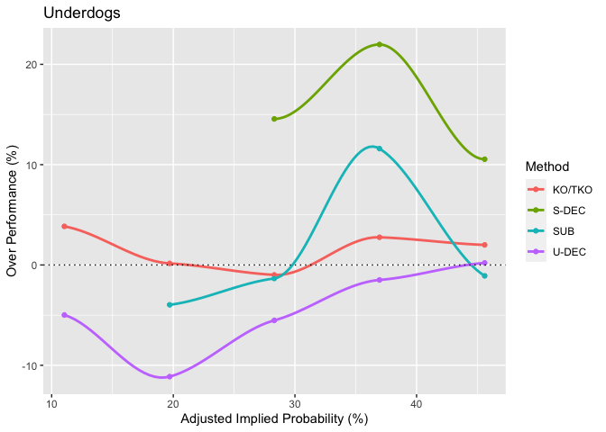
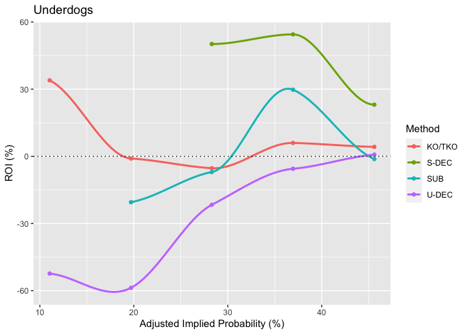
Does the method of victory affect the relationship between odds and outcome? Reduce number of bins (compared to Year comparison above) to stabilize estimates. Graphs do not tell whole story due to number of data points available across bins.

odds_perf_by_method = gauge_over_performance(num_bin = 5, min_bin_size = 30, variable = "Method")

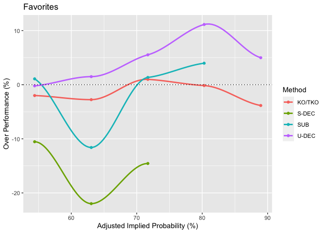
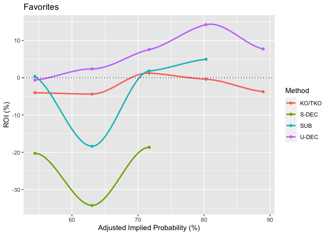
kable(odds_perf_by_method)

Probability_Bin	Dummy	Prop_of_Victory	Size_of_Bin	ROI	Mid_Bin	Over_Performance	Is_Fav
(0.501,0.587]	KO/TKO	0.5240000	250	-0.0403200	0.54400	-0.0200000	TRUE
(0.501,0.587]	M-DEC	0.6666667	9	0.1844444	0.54400	0.1226667	TRUE
(0.501,0.587]	S-DEC	0.4385965	114	-0.2028947	0.54400	-0.1054035	TRUE
(0.501,0.587]	SUB	0.5548387	155	0.0037419	0.54400	0.0108387	TRUE
(0.501,0.587]	U-DEC	0.5419162	334	-0.0062874	0.54400	-0.0020838	TRUE
(0.587,0.674]	KO/TKO	0.6028881	277	-0.0437906	0.63050	-0.0276119	TRUE
(0.587,0.674]	M-DEC	0.6666667	6	0.0666667	0.63050	0.0361667	TRUE
(0.587,0.674]	S-DEC	0.4107143	112	-0.3425893	0.63050	-0.2197857	TRUE
(0.587,0.674]	SUB	0.5144928	138	-0.1839130	0.63050	-0.1160072	TRUE
(0.587,0.674]	U-DEC	0.6454294	361	0.0236842	0.63050	0.0149294	TRUE
(0.674,0.76]	KO/TKO	0.7268722	227	0.0123789	0.71700	0.0098722	TRUE
(0.674,0.76]	M-DEC	0.0000000	1	-1.0000000	0.71700	-0.7170000	TRUE
(0.674,0.76]	S-DEC	0.5714286	63	-0.1866667	0.71700	-0.1455714	TRUE
(0.674,0.76]	SUB	0.7304348	115	0.0180000	0.71700	0.0134348	TRUE
(0.674,0.76]	U-DEC	0.7722420	281	0.0755516	0.71700	0.0552420	TRUE
(0.76,0.846]	KO/TKO	0.8014184	141	-0.0039716	0.80300	-0.0015816	TRUE
(0.76,0.846]	M-DEC	1.0000000	1	0.2600000	0.80300	0.1970000	TRUE
(0.76,0.846]	S-DEC	0.4500000	20	-0.4270000	0.80300	-0.3530000	TRUE
(0.76,0.846]	SUB	0.8426966	89	0.0495506	0.80300	0.0396966	TRUE
(0.76,0.846]	U-DEC	0.9142857	140	0.1424286	0.80300	0.1112857	TRUE
(0.846,0.933]	KO/TKO	0.8510638	47	-0.0374468	0.88950	-0.0384362	TRUE
(0.846,0.933]	S-DEC	1.0000000	3	0.1533333	0.88950	0.1105000	TRUE
(0.846,0.933]	SUB	0.9583333	24	0.0820833	0.88950	0.0688333	TRUE
(0.846,0.933]	U-DEC	0.9393939	33	0.0772727	0.88950	0.0498939	TRUE
(0.0669,0.154]	KO/TKO	0.1489362	47	0.3393617	0.11045	0.0384862	FALSE
(0.0669,0.154]	S-DEC	0.0000000	3	-1.0000000	0.11045	-0.1104500	FALSE
(0.0669,0.154]	SUB	0.0416667	24	-0.7025000	0.11045	-0.0687833	FALSE
(0.0669,0.154]	U-DEC	0.0606061	33	-0.5239394	0.11045	-0.0498439	FALSE
(0.154,0.24]	KO/TKO	0.1985816	141	-0.0098582	0.19700	0.0015816	FALSE
(0.154,0.24]	M-DEC	0.0000000	1	-1.0000000	0.19700	-0.1970000	FALSE
(0.154,0.24]	S-DEC	0.5500000	20	1.6125000	0.19700	0.3530000	FALSE
(0.154,0.24]	SUB	0.1573034	89	-0.2049438	0.19700	-0.0396966	FALSE
(0.154,0.24]	U-DEC	0.0857143	140	-0.5875714	0.19700	-0.1112857	FALSE
(0.24,0.326]	KO/TKO	0.2731278	227	-0.0531718	0.28300	-0.0098722	FALSE
(0.24,0.326]	M-DEC	1.0000000	1	2.0300000	0.28300	0.7170000	FALSE
(0.24,0.326]	S-DEC	0.4285714	63	0.5015873	0.28300	0.1455714	FALSE
(0.24,0.326]	SUB	0.2695652	115	-0.0703478	0.28300	-0.0134348	FALSE
(0.24,0.326]	U-DEC	0.2277580	281	-0.2165836	0.28300	-0.0552420	FALSE
(0.326,0.413]	KO/TKO	0.3971119	277	0.0597473	0.36950	0.0276119	FALSE
(0.326,0.413]	M-DEC	0.3333333	6	-0.0916667	0.36950	-0.0361667	FALSE
(0.326,0.413]	S-DEC	0.5892857	112	0.5446429	0.36950	0.2197857	FALSE
(0.326,0.413]	SUB	0.4855072	138	0.2974638	0.36950	0.1160072	FALSE
(0.326,0.413]	U-DEC	0.3545706	361	-0.0556510	0.36950	-0.0149294	FALSE
(0.413,0.499]	KO/TKO	0.4760000	250	0.0419600	0.45600	0.0200000	FALSE
(0.413,0.499]	M-DEC	0.3333333	9	-0.2344444	0.45600	-0.1226667	FALSE
(0.413,0.499]	S-DEC	0.5614035	114	0.2307018	0.45600	0.1054035	FALSE
(0.413,0.499]	SUB	0.4451613	155	-0.0121935	0.45600	-0.0108387	FALSE
(0.413,0.499]	U-DEC	0.4580838	334	0.0074251	0.45600	0.0020838	FALSE

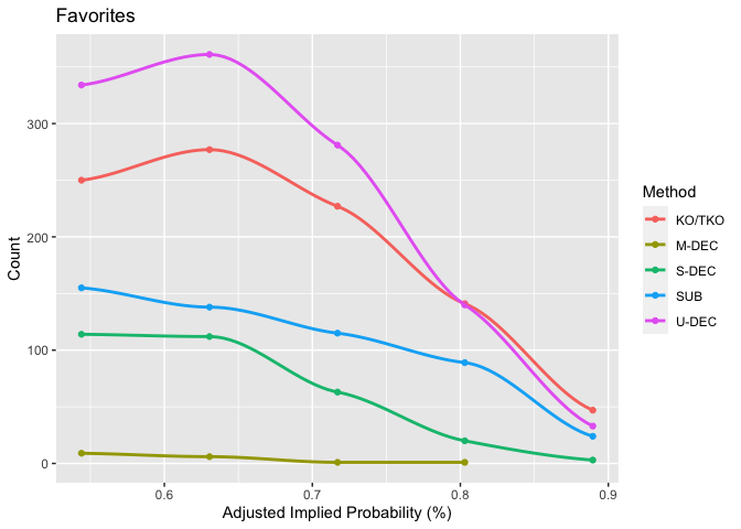
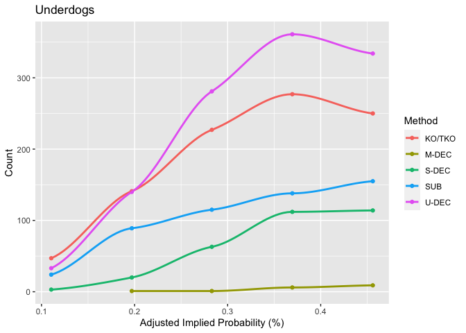
How does fight finishing method vary with implied probability of vegas odds?

odds_perf_by_method %>%
  dplyr::filter(Is_Fav == T) %>%
  ggplot(aes(x=Mid_Bin, y=Size_of_Bin, group = Dummy, color = Dummy))+
  geom_point()+
  geom_smooth(se=F)+
  ylab("Count")+
  xlab("Adjusted Implied Probability (%)")+
  ggtitle("Favorites")+
  labs(color="Method")

odds_perf_by_method %>%
  dplyr::filter(Is_Fav == F) %>%
  ggplot(aes(x=Mid_Bin, y=Size_of_Bin, group = Dummy, color = Dummy))+
  geom_point()+
  geom_smooth(se=F)+
  ylab("Count")+
  xlab("Adjusted Implied Probability (%)")+
  ggtitle("Underdogs")+
  labs(color="Method")

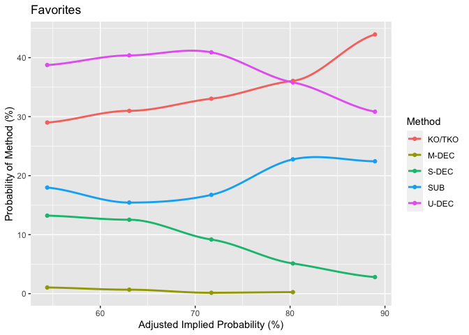
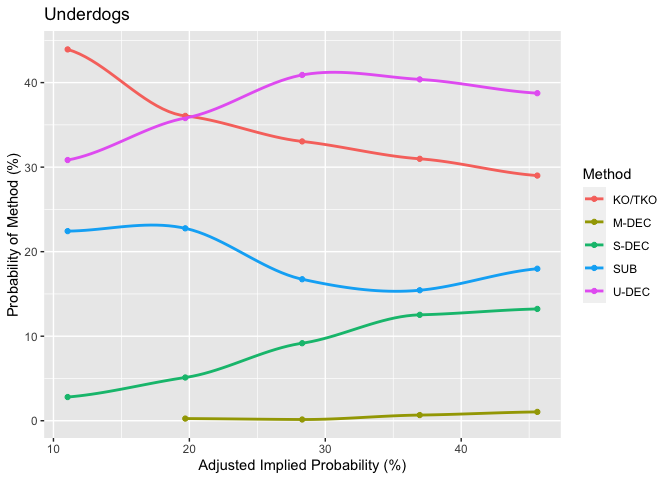
Calculate the proportion of fights that end by various methods as a function of implied probability of fight odds.

odds_perf_by_method %>%
  group_by(Is_Fav, Mid_Bin) %>%
  summarise(Total_Count = sum(Size_of_Bin)) -> total_count

odds_perf_by_method %>%
  group_by(Is_Fav, Mid_Bin, Dummy) %>%
  summarise(Count= Size_of_Bin) -> single_count

method_count_by_odds = merge(single_count, total_count)
method_count_by_odds %>%
  dplyr::mutate(Method_Prop = Count / Total_Count ) -> method_count_by_odds

method_count_by_odds %>%
  dplyr::filter(Is_Fav == T) %>%
  ggplot(aes(x=Mid_Bin*100, y=Method_Prop*100, group = Dummy, color=Dummy))+
  geom_point()+
  geom_smooth(se=F)+
  ylab("Probability of Method (%)")+
  xlab("Adjusted Implied Probability (%)")+
  ggtitle("Favorites")+
  labs(color="Method")

method_count_by_odds %>%
  dplyr::filter(Is_Fav == F) %>%
  ggplot(aes(x=Mid_Bin*100, y=Method_Prop*100, group = Dummy, color=Dummy))+
  geom_point()+
  geom_smooth(se=F)+
  ylab("Probability of Method (%)")+
  xlab("Adjusted Implied Probability (%)")+
  ggtitle("Underdogs")+
  labs(color="Method")

Fighter Odds

Convert short back to long format.

df_odds_short %>%
  gather(key = "Result", value = "NAME", Loser:Winner) -> df_odds_long

Identify if fighter was favortie to assign proper Implied Probability.

df_odds_long %>%
  dplyr::mutate(
  Was_Favorite = ifelse(
    (Favorite_was_Winner & (Result == "Winner")) | (!Favorite_was_Winner & (Result == "Loser"))
    , T
    , F
  )
) -> df_odds_long

summary(df_odds_long[, "Was_Favorite"])

##    Mode   FALSE    TRUE 
## logical    2941    2941

Identify Implied Probability of each fighter.

df_odds_long %>%
  dplyr::mutate(
    Implied_Probability = ifelse(
      Was_Favorite
      , Favorite_Probability
      , Underdog_Probability
    )
    , Adjusted_Implied_Probability = ifelse(
      Was_Favorite
      , Adjusted_Favorite_Probability
      , Adjusted_Underdog_Probability
    )
  ) -> df_odds_long

summary(df_odds_long[,c("Implied_Probability", "Adjusted_Implied_Probability")])

##  Implied_Probability Adjusted_Implied_Probability
##  Min.   :0.07117     Min.   :0.0673              
##  1st Qu.:0.35971     1st Qu.:0.3593              
##  Median :0.50000     Median :0.5000              
##  Mean   :0.50223     Mean   :0.5000              
##  3rd Qu.:0.64103     3rd Qu.:0.6407              
##  Max.   :0.94340     Max.   :0.9327

Get rid of useless columns.

df_odds_long %>% dplyr::select(
  c(
    NAME
    , Event
    , Date
    , Result
    , Implied_Probability
    , Adjusted_Implied_Probability
  )
) -> df_odds_long

Summarize data.

summary(df_odds_long)

##      NAME                                            Event     
##  Length:5882        UFC Fight Night: Chiesa vs. Magny   :  28  
##  Class :character   UFC Fight Night: Poirier vs. Gaethje:  28  
##  Mode  :character   UFC Fight Night: Whittaker vs. Till :  28  
##                     UFC 190: Rousey vs Correia          :  26  
##                     UFC 193: Rousey vs Holm             :  26  
##                     UFC 210: Cormier vs. Johnson 2      :  26  
##                     (Other)                             :5720  
##       Date               Result          Implied_Probability
##  Min.   :2013-04-27   Length:5882        Min.   :0.07117    
##  1st Qu.:2015-08-23   Class :character   1st Qu.:0.35971    
##  Median :2017-05-13   Mode  :character   Median :0.50000    
##  Mean   :2017-06-17                      Mean   :0.50223    
##  3rd Qu.:2019-04-20                      3rd Qu.:0.64103    
##  Max.   :2021-02-06                      Max.   :0.94340    
##                                                             
##  Adjusted_Implied_Probability
##  Min.   :0.0673              
##  1st Qu.:0.3593              
##  Median :0.5000              
##  Mean   :0.5000              
##  3rd Qu.:0.6407              
##  Max.   :0.9327              
## 

Add Win and Log Odds columns.

df_odds_long %>%
  dplyr::mutate(
    Won = ifelse(Result == "Winner", T, F)
    , Logit_Prob = qlogis(Implied_Probability)
    , Adjusted_Logit_Prob = qlogis(Adjusted_Implied_Probability)
  ) -> df_odds_long

summary(df_odds_long[, c("Won", "Logit_Prob", "Adjusted_Logit_Prob")])

##     Won            Logit_Prob       Adjusted_Logit_Prob
##  Mode :logical   Min.   :-2.56879   Min.   :-2.6289    
##  FALSE:2941      1st Qu.:-0.57661   1st Qu.:-0.5786    
##  TRUE :2941      Median : 0.00000   Median : 0.0000    
##                  Mean   : 0.01186   Mean   : 0.0000    
##                  3rd Qu.: 0.57982   3rd Qu.: 0.5786    
##                  Max.   : 2.81341   Max.   : 2.6289

Get performance and odds for each fighter using Adjusted Implied Probability.

df_odds_long %>%
  dplyr::group_by(NAME) %>%
  dplyr::summarise(
    Exp_Prop = mean(Adjusted_Implied_Probability)
    , Logit_Exp_Prop = mean(Adjusted_Logit_Prob)
    , Win_Prop = mean(Won)
    , N_Fights = length(Won)
    , Over_Performance = Win_Prop - Exp_Prop
    , Logit_Over = qlogis(Win_Prop) - Logit_Exp_Prop
    , Back_Trans_Exp = plogis(Logit_Exp_Prop)
  ) -> df_odds_long_fighters

Look at which fights were included in the dataset for a specific fighter.

df_odds_long %>%
  dplyr::filter(NAME == "Roxanne Modafferi") -> df_roxy

kable(df_roxy)

NAME	Event	Date	Result	Implied_Probability	Adjusted_Implied_Probability	Won	Logit_Prob	Adjusted_Logit_Prob
Roxanne Modafferi	UFC Fight Night: Dos Anjos vs. Edwards	2019-07-20	Loser	0.4385965	0.4399686	FALSE	-0.2468601	-0.2412893
Roxanne Modafferi	UFC Fight Night: Blaydes vs. Volkov	2020-06-20	Loser	0.4651163	0.4694002	FALSE	-0.1397619	-0.1225522
Roxanne Modafferi	The Ultimate Fighter: Team Rousey vs. Team Tate Finale	2013-11-30	Loser	0.1937984	0.2000738	FALSE	-1.4255151	-1.3858330
Roxanne Modafferi	UFC Fight Night: Chiesa vs. Magny	2021-01-20	Loser	0.2777778	0.2657546	FALSE	-0.9555114	-1.0162702
Roxanne Modafferi	UFC 230: Cormier vs. Lewis	2018-11-03	Loser	0.1724138	0.1695402	FALSE	-1.5686159	-1.5888892
Roxanne Modafferi	UFC Fight Night: Waterson vs. Hill	2020-09-12	Winner	0.2777778	0.2657546	TRUE	-0.9555114	-1.0162702
Roxanne Modafferi	UFC Fight Night: Overeem vs. Oleinik	2019-04-20	Winner	0.2666667	0.2683698	TRUE	-1.0116009	-1.0029092
Roxanne Modafferi	UFC 246: McGregor vs. Cowboy	2020-01-18	Winner	0.1246883	0.1159156	TRUE	-1.9487632	-2.0316905

Top 10 over-performers with at least 5 fights where number of fights is simply number available in the dataset (see above).

df_odds_long_fighters %>%
  dplyr::filter(N_Fights >= 5) %>%
  dplyr::arrange(desc(Over_Performance)) %>%
  head(10) -> df_top_over_perform
# now with logit
df_odds_long_fighters %>%
  dplyr::filter(N_Fights >= 5) %>%
  dplyr::arrange(desc(Logit_Over)) %>%
  head(10) -> df_top_over_perform_logit

kable(df_top_over_perform, caption = "Top 10 Over Performers with at least 5 Fights")  

Top 10 Over Performers with at least 5 Fights

NAME	Exp_Prop	Logit_Exp_Prop	Win_Prop	N_Fights	Over_Performance	Logit_Over	Back_Trans_Exp
Leonardo Santos	0.4454486	-0.2777403	1.0000000	5	0.5545514	Inf	0.4310079
Robert Whittaker	0.4996490	0.0065223	1.0000000	10	0.5003510	Inf	0.5016306
Brandon Moreno	0.4399010	-0.2686787	0.8571429	7	0.4172418	2.060438	0.4332315
Arnold Allen	0.5867006	0.3757653	1.0000000	6	0.4132994	Inf	0.5928513
Brian Ortega	0.4823820	-0.0684020	0.8750000	8	0.3926180	2.014312	0.4829062
Alexander Volkanovski	0.6101305	0.5177296	1.0000000	8	0.3898695	Inf	0.6266167
Bryan Caraway	0.4194964	-0.3415057	0.8000000	5	0.3805036	1.727800	0.4154438
Yan Xiaonan	0.6240270	0.5391744	1.0000000	5	0.3759730	Inf	0.6316203
Amanda Nunes	0.5507052	0.2811614	0.9166667	12	0.3659615	2.116734	0.5698309
Joaquim Silva	0.4575904	-0.1889315	0.8000000	5	0.3424096	1.575226	0.4529071

kable(df_top_over_perform_logit, caption = "Logit Scale: Top 10 Over Performers with at least 5 Fights")

Logit Scale: Top 10 Over Performers with at least 5 Fights

NAME	Exp_Prop	Logit_Exp_Prop	Win_Prop	N_Fights	Over_Performance	Logit_Over	Back_Trans_Exp
Alexander Volkanovski	0.6101305	0.5177296	1	8	0.3898695	Inf	0.6266167
Arnold Allen	0.5867006	0.3757653	1	6	0.4132994	Inf	0.5928513
Demetrious Johnson	0.8609483	1.8803058	1	9	0.1390517	Inf	0.8676462
Israel Adesanya	0.7002859	0.8678323	1	7	0.2997141	Inf	0.7042944
Jon Jones	0.7892464	1.3952860	1	7	0.2107536	Inf	0.8014348
Kamaru Usman	0.6925314	0.8901129	1	10	0.3074686	Inf	0.7089135
Khabib Nurmagomedov	0.7598282	1.2002959	1	9	0.2401718	Inf	0.7685774
Kyung Ho Kang	0.6633446	0.7104716	1	6	0.3366554	Inf	0.6705054
Leonardo Santos	0.4454486	-0.2777403	1	5	0.5545514	Inf	0.4310079
Petr Yan	0.8144451	1.5256823	1	5	0.1855549	Inf	0.8213737

Top 10 under performers with at least 5 fights.

df_odds_long_fighters %>%
  dplyr::filter(N_Fights >= 5) %>%
  dplyr::arrange(Over_Performance) %>%
  head(10) -> df_top_under_perform
# with logit
df_odds_long_fighters %>%
  dplyr::filter(N_Fights >= 5) %>%
  dplyr::arrange(Logit_Over) %>%
  head(10) -> df_top_under_perform_logit

kable(df_top_under_perform, caption = "Top 10 Under Performers with at least 5 Fights")

Top 10 Under Performers with at least 5 Fights

NAME	Exp_Prop	Logit_Exp_Prop	Win_Prop	N_Fights	Over_Performance	Logit_Over	Back_Trans_Exp
Kailin Curran	0.5404624	0.1811195	0.1428571	7	-0.3976052	-1.972879	0.5451565
Joshua Burkman	0.3760531	-0.5400292	0.0000000	7	-0.3760531	-Inf	0.3681808
Hyun Gyu Lim	0.5720479	0.3587458	0.2000000	5	-0.3720479	-1.745040	0.5887368
Alexander Gustafsson	0.6271431	0.5898086	0.2857143	7	-0.3414288	-1.506099	0.6433212
Gray Maynard	0.5072171	0.0245074	0.1666667	6	-0.3405504	-1.633945	0.5061265
Junior Albini	0.5325358	0.1453508	0.2000000	5	-0.3325358	-1.531645	0.5362739
Rashad Evans	0.5236378	0.1041933	0.2000000	5	-0.3236378	-1.490488	0.5260248
Andrea Lee	0.7055647	0.8841184	0.4000000	5	-0.3055647	-1.289583	0.7076749
Johny Hendricks	0.5509110	0.2250002	0.2500000	8	-0.3009110	-1.323613	0.5560140
Anderson Silva	0.4249640	-0.3485824	0.1428571	7	-0.2821068	-1.443177	0.4137262

kable(df_top_under_perform_logit, caption ="Logit Scale: Top 10 Under Performers with at least 5 Fights" )

Logit Scale: Top 10 Under Performers with at least 5 Fights

NAME	Exp_Prop	Logit_Exp_Prop	Win_Prop	N_Fights	Over_Performance	Logit_Over	Back_Trans_Exp
Joshua Burkman	0.3760531	-0.5400292	0.0000000	7	-0.3760531	-Inf	0.3681808
Kailin Curran	0.5404624	0.1811195	0.1428571	7	-0.3976052	-1.972879	0.5451565
Hyun Gyu Lim	0.5720479	0.3587458	0.2000000	5	-0.3720479	-1.745040	0.5887368
Gray Maynard	0.5072171	0.0245074	0.1666667	6	-0.3405504	-1.633945	0.5061265
Junior Albini	0.5325358	0.1453508	0.2000000	5	-0.3325358	-1.531645	0.5362739
Alexander Gustafsson	0.6271431	0.5898086	0.2857143	7	-0.3414288	-1.506099	0.6433212
Rashad Evans	0.5236378	0.1041933	0.2000000	5	-0.3236378	-1.490488	0.5260248
Anderson Silva	0.4249640	-0.3485824	0.1428571	7	-0.2821068	-1.443177	0.4137262
Ronda Rousey	0.8322407	1.8077087	0.6000000	5	-0.2322407	-1.402244	0.8590847
Brad Pickett	0.3826965	-0.5461462	0.1250000	8	-0.2576965	-1.399764	0.3667590

Most favored fighters with at least 5 fights

df_odds_long_fighters %>%
  dplyr::filter(N_Fights >= 5) %>%
  dplyr::arrange(desc(Exp_Prop)) %>%
  head(10) -> df_most_fav
# with logit
df_odds_long_fighters %>%
  dplyr::filter(N_Fights >= 5) %>%
  dplyr::arrange(desc(Logit_Exp_Prop)) %>%
  head(10) -> df_most_fav_logit

kable(df_most_fav)

NAME	Exp_Prop	Logit_Exp_Prop	Win_Prop	N_Fights	Over_Performance	Logit_Over	Back_Trans_Exp
Demetrious Johnson	0.8609483	1.880306	1.0000000	9	0.1390517	Inf	0.8676462
Ronda Rousey	0.8322407	1.807709	0.6000000	5	-0.2322407	-1.4022436	0.8590847
Cristiane Justino	0.8252814	1.703941	0.8571429	7	0.0318615	0.0878185	0.8460487
Petr Yan	0.8144451	1.525682	1.0000000	5	0.1855549	Inf	0.8213737
Zabit Magomedsharipov	0.8050291	1.485833	1.0000000	6	0.1949709	Inf	0.8154520
Tatiana Suarez	0.7972730	1.391506	1.0000000	5	0.2027270	Inf	0.8008325
Jon Jones	0.7892464	1.395286	1.0000000	7	0.2107536	Inf	0.8014348
Magomed Ankalaev	0.7647264	1.211622	0.8000000	5	0.0352736	0.1746719	0.7705859
Khabib Nurmagomedov	0.7598282	1.200296	1.0000000	9	0.2401718	Inf	0.7685774
Mairbek Taisumov	0.7342042	1.072182	0.7777778	9	0.0435736	0.1805805	0.7450117

kable(df_most_fav_logit)

NAME	Exp_Prop	Logit_Exp_Prop	Win_Prop	N_Fights	Over_Performance	Logit_Over	Back_Trans_Exp
Demetrious Johnson	0.8609483	1.880306	1.0000000	9	0.1390517	Inf	0.8676462
Ronda Rousey	0.8322407	1.807709	0.6000000	5	-0.2322407	-1.4022436	0.8590847
Cristiane Justino	0.8252814	1.703941	0.8571429	7	0.0318615	0.0878185	0.8460487
Petr Yan	0.8144451	1.525682	1.0000000	5	0.1855549	Inf	0.8213737
Zabit Magomedsharipov	0.8050291	1.485833	1.0000000	6	0.1949709	Inf	0.8154520
Jon Jones	0.7892464	1.395286	1.0000000	7	0.2107536	Inf	0.8014348
Tatiana Suarez	0.7972730	1.391506	1.0000000	5	0.2027270	Inf	0.8008325
Magomed Ankalaev	0.7647264	1.211622	0.8000000	5	0.0352736	0.1746719	0.7705859
Khabib Nurmagomedov	0.7598282	1.200296	1.0000000	9	0.2401718	Inf	0.7685774
Mairbek Taisumov	0.7342042	1.072182	0.7777778	9	0.0435736	0.1805805	0.7450117

Least favored fighters with at least 5 fights.

df_odds_long_fighters %>%
  dplyr::filter(N_Fights >= 5) %>%
  dplyr::arrange(Exp_Prop) %>%
  head(10) -> df_least_fav
# with logit
df_odds_long_fighters %>%
  dplyr::filter(N_Fights >= 5) %>%
  dplyr::arrange(Logit_Exp_Prop) %>%
  head(10) -> df_least_fav_logit

kable(df_least_fav, caption = "Top 10 Least Favored Fighters with at least 5 Fights")

Top 10 Least Favored Fighters with at least 5 Fights

NAME	Exp_Prop	Logit_Exp_Prop	Win_Prop	N_Fights	Over_Performance	Logit_Over	Back_Trans_Exp
Roxanne Modafferi	0.2743472	-1.0507130	0.3750000	8	0.1006528	0.5398874	0.2590882
Daniel Kelly	0.2769185	-0.9737988	0.6000000	10	0.3230815	1.3792639	0.2741240
Jessica Aguilar	0.2859562	-0.9707245	0.2000000	5	-0.0859562	-0.4155698	0.2747361
Dan Henderson	0.2887631	-0.9309147	0.5000000	6	0.2112369	0.9309147	0.2827392
Thibault Gouti	0.2982523	-0.9293738	0.1666667	6	-0.1315857	-0.6800641	0.2830518
Anthony Perosh	0.2985353	-0.9384366	0.4000000	5	0.1014647	0.5329715	0.2812162
Leslie Smith	0.3018944	-0.9783537	0.4000000	5	0.0981056	0.5728886	0.2732186
Garreth McLellan	0.3067211	-0.8343938	0.2000000	5	-0.1067211	-0.5519005	0.3027168
Yaotzin Meza	0.3076578	-0.8634526	0.4000000	5	0.0923422	0.4579875	0.2966185
Takanori Gomi	0.3093210	-0.8732262	0.2000000	5	-0.1093210	-0.5130682	0.2945834

kable(df_least_fav_logit, caption = "Logit Scale: Top 10 Least Favored Fighters with at least 5 Fights")

Logit Scale: Top 10 Least Favored Fighters with at least 5 Fights

NAME	Exp_Prop	Logit_Exp_Prop	Win_Prop	N_Fights	Over_Performance	Logit_Over	Back_Trans_Exp
Roxanne Modafferi	0.2743472	-1.0507130	0.3750000	8	0.1006528	0.5398874	0.2590882
Leslie Smith	0.3018944	-0.9783537	0.4000000	5	0.0981056	0.5728886	0.2732186
Daniel Kelly	0.2769185	-0.9737988	0.6000000	10	0.3230815	1.3792639	0.2741240
Jessica Aguilar	0.2859562	-0.9707245	0.2000000	5	-0.0859562	-0.4155698	0.2747361
Anthony Perosh	0.2985353	-0.9384366	0.4000000	5	0.1014647	0.5329715	0.2812162
Dan Henderson	0.2887631	-0.9309147	0.5000000	6	0.2112369	0.9309147	0.2827392
Thibault Gouti	0.2982523	-0.9293738	0.1666667	6	-0.1315857	-0.6800641	0.2830518
Takanori Gomi	0.3093210	-0.8732262	0.2000000	5	-0.1093210	-0.5130682	0.2945834
Yaotzin Meza	0.3076578	-0.8634526	0.4000000	5	0.0923422	0.4579875	0.2966185
Julian Erosa	0.3202609	-0.8581763	0.2000000	5	-0.1202609	-0.5281181	0.2977205

Examine odds for specific fighters.

# Israel Adesanya
df_odds_long_fighters %>% dplyr::filter(NAME == "Israel Adesanya") -> df_Izzy
kable(df_Izzy)

NAME	Exp_Prop	Logit_Exp_Prop	Win_Prop	N_Fights	Over_Performance	Logit_Over	Back_Trans_Exp
Israel Adesanya	0.7002859	0.8678323	1	7	0.2997141	Inf	0.7042944

# Anthony Smith
df_odds_long_fighters %>% dplyr::filter(NAME == "Anthony Smith") -> df_Smith
kable(df_Smith)

NAME	Exp_Prop	Logit_Exp_Prop	Win_Prop	N_Fights	Over_Performance	Logit_Over	Back_Trans_Exp
Anthony Smith	0.4539811	-0.2286408	0.6428571	14	0.1888761	0.8164275	0.4430875